Physical Modeling and Measurement of Fish Acoustic Backscatter

(1)

Physical modeling and measurement of fish acoustic backscatter

Henry M. Manik

Citation: AIP Conf. Proc. 1454, 99 (2012); doi: 10.1063/1.4730697 View online: http://dx.doi.org/10.1063/1.4730697

View Table of Contents: http://proceedings.aip.org/dbt/dbt.jsp?KEY=APCPCS&Volume=1454&Issue=1 Published by the American Institute of Physics.

Additional information on AIP Conf. Proc.

Journal Homepage: http://proceedings.aip.org/

Journal Information: http://proceedings.aip.org/about/about_the_proceedings

(2)

Physical Modeling and Measurement of Fish

Acoustic Backscatter

Henry M. Manik

Laboratory of Ocean Acoustic and Instrumentation Department of Marine Science and Technology Faculty of Fisheries and Marine Sciences Bogor Agricultural University Kampus IPB Darmaga Bogor 16680

Indonesia E-mail : henrymanik@ipb.ac.id

Abstract. Physical acoustic model of fish is used to explain the variability in backscatter and target size. The research has the aim to apply the theoretical physics-based acoustic scattering models of single animal and laboratory measurements of backscattering by individual fish. The scattering process was modeled using the distorted-wave Born approximation. Results showed that the acoustic backscatter strongly depended on the fish orientation. Predicted scattering over the measured distribution of orientations resulted in predictions of target strength consistent with measurements of target strength of fish.

Keywords: physical model, fish, acoustic backscatter

PACS: 43.30.Sf

INTRODUCTION

Acoustic technology has been extensively used for surveys of fish biomass [1, 2]. Acoustical methods for measuring distribution and stock have several advantages over the more traditional net sampling. Acoustics can provide real time estimates of abundance, whereas estimates from net samples are normally made after the cruise. Net sampling skews biomass estimates in favor of those species that are poor avoiders [3]. Nets integrate stock over the distance they are open, thereby decreasing their ability to resolve spatial variability. In contrast, acoustic methods can resolve spatial variability on the order of 1 m [4].

Acoustical methods work by transmitting pulses of sound into the seawater and measuring the backscattering energy (echo) as a function of time or depth. The conversion of the acoustic backscattered energy to fish numerical density is based on two steps. First, it is assumed that the efficiency with which an fish scatters sound is quantifiable and is a function of the acoustic frequency and the fish’s length, shape, tilt angle, and material properties. This scattering efficiency is normally represented by the fish backscattering cross-section σbs, with units of area or

target strength TS, in decibels [5].

Second, the energy backscattered from a collection of fish is equal to the sum of the energy echoed by each fish [6]. This is determined using the sonar equation [7] and the volume backscattering strength (SV). SV is the logarithmic equivalent of the volume backscattering coefficient Sv, whose units are m-1 [4]. This paper describes a study of acoustic backscattering from fish at 200 kHz frequency as a function of fish orientation. The measurements were compared with predictions using the physics based

acoustic scattering Distorted Wave Born

Approximation (DWBA) model.

MATERIAL AND METHODS

Experimental Design

Fish samples were collected from Pelabuhan Ratu Bay and transported by car to the campus of Bogor Agricultural University. The laboratory experiment were conducted at the water tank of ocean acoustic laboratory Bogor Agricultural University.

(3)

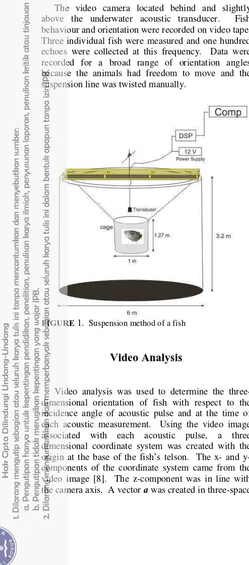
fish were placed using a vertical tether of 0.15 mm diameter monofilament (Fig. 1). The animal was tied with a 50 µm diameter syntetic line around the first abdominal segment. This tethering scheme kept it within the acoustic beam, but permitted considerable freedom of movement and orientation.

The acoustic system was calibrated to measure the transmitting and receiving value of tranducer. All 200 kHz data were processed to determine target strengths form each fish echo.

The video camera located behind and slightly above the underwater acoustic transducer. Fish behaviour and orientation were recorded on video tape. Three individual fish were measured and one hundred echoes were collected at this frequency. Data were recorded for a broad range of orientation angles because the animals had freedom to move and the suspension line was twisted manually.

FIGURE 1. Suspension method of a fish

Video Analysis

Video analysis was used to determine the three-dimensional orientation of fish with respect to the incidence angle of acoustic pulse and at the time of each acoustic measurement. Using the video image associated with each acoustic pulse, a three dimensional coordinate system was created with the origin at the base of the fish’s telson. The x- and y- components of the coordinate system came from the video image [8]. The z-component was in line with the camera axis. A vector a was created in three-space

going from the origin to a point midway between the

eyes. The length

a

of a was found by measuring the projection from an image where the fish was believed to be parallel to the image plane. The angle β was the angle between a and its projection onto the

image plane such that

β

=

cos

−1

(

a

_x2

+

a

_y2

/

a

).

The x- and y-components of a came from the video image. The z-component was derived from

.

sin

β

a

_z

=

The acoustic wave number vector k

had a direction from the z-axis and magnitude

λ

π

/

2

=

k

, where λ was the acoustic wavelength in water. Therefore,













=













=

θ

cos

0

sin

ˆ

k

z y x (1) meas

φ

was the angle measuring the orientation of the fish relative to the direction of acoustic incidence, determined using the dot product of the two vectors k

and a [8] :













=

−

a

k

a

k

meas

.

cos

1

φ

(2)

Physical Modeling

Acoustic scattering from a three-dimensional object having density and sound speed close to those of the surrounding medium can be modeled using the Distorted Wave Born Approximation (DWBA) [9]. A DWBA model is composed of the following volume integral :

=

∫∫ ∫

−

V r k i

bs

e

dV

k

f

1 2.0

2

1

(

)

4

π

γ

κ

γ

ρ (3) where fbs is the complex backscattering amplitude,

related to σbs by the relationship

2

bs bs

=

f

σ

; k is the

acoustic wave number given by k = 2π /λ, where λ is the acoustic wave length;

γ

_k

=

(

κ

₂

−

κ

₁

)

where κ is [image:3.612.46.293.198.758.2]

(4)

density; c is sound speed; r0 is the position vector. The

subscript 1 refers to the ambient seawater and the subscript 2 refers to the fish scattering the sound.

In the case of a uniformly bent cylinder with radius of curvature ρc, Stanton et al. (1998) give the expression for the scattering amplitude

(4) where k is the acoustic wave number in the surrounding seawater (subscript 1)and the fish body (subscript 2); γk and γρ are related to densities (ρ) and sound speeds (c) of surrounding seawater (1) and fish body (2) following (γk = κ2 – κ1)/ κ1 and (γρ = ρ2 - ρ1)/

ρ2 , and κ =(ρc2) -1, where κis compressibility; J1 is a Bessel function of the first kind of order 1; βtilt is the angle between the incident wave (ki) and the cross section of the cylinder at each point along its axis [10]. The Target Strength (TS) is quantified by

TS

=

10

log

₁₀

(

f

_bs2

).

(5)

RESULTS AND DISCUSSION

Figure 2 shows the relation of target strength and fish size. The increasing of fish size is followed by increasing target strength value. Density and sound speed contrast (g and h) were assumed to be constant throughout the fish. Values for these were taken from [7] for fish : g = 1.1347, h = 1.1279. The 180o acoustic backscattering pattern of the fish was callculated in 1o increments. This was done starting with a wave number vector k1 pointing at an angle of

φDWBA = 0o. Acoustic backscattering cross section σbs

and target strength (TS) against angle of incidence are shown in Fig. 3a and 3b.

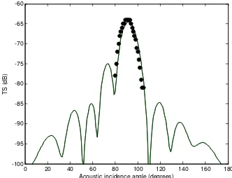
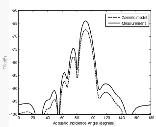
Models and measurements were shifted into the same reference frame and plotted together for comparison (Fig. 4). The experimentally measured scattering pattern showed the highest levels of scattering at incidence angless close to 90o. This being said, the measurements appear generally to confirm the models, with main lobes in the scattering pattern at similar angles. The DWBA model depends upon a coherent summation of scattering from a volume. Figure 5 shows the measured TS pattern of the fish were in reasonable agreement with the theoretical TS patterns. We had confirmed, therefore, that our measurement system were able to quantify precisely the TS patterns of fish.

FIGURE 2. Target strength in relation to fish size.

0 50 100 150 180 0 0.2 0.4 0.6 0.8 1 1.2 1.4 1.6 1.8

2x 10

-7

Acoustic incidence angle (degrees)

A c o us ti c ba c k s c a tt e ri n g c ro s s s e c ti o n (m 2)

0 50 100 150 180 -100 -95 -90 -85 -80 -75 -70 -65 -60

T a rg et S tr en g th ( d B )

(a) (b) FIGURE 3. Steps in forming a Distorted Wave Born Approximation (DWBA) model of fish. (a) Backscattering

cross-section (σbs) vs. angle of incidence. (b) Target

strength vs. angle of incidence. The peak in the scattering pattern occur at angles close to dorsal aspect.

0 20 40 60 80 100 120 140 160 180

-100 -95 -90 -85 -80 -75 -70 -65 -60

T S ( d B )

FIGURE 4. TS pattern from measurements (•), and DWBA

model calculations ().

[image:4.612.317.526.101.223.2] [image:4.612.326.514.252.415.2] [image:4.612.323.489.488.615.2]

(5)

0 20 40 60 80 100 120 140 160 180 -100

-95 -90 -85 -80 -75 -70 -65 -60

Acoustic Incidence Angle (degrees)

T

S

(

d

B

)

Generic model Measurement

FIGURE 5. TS pattern from measurements (---) and

DWBA model calculations ().

CONCLUSIONS

A new Target Strength (TS) measurement method using a single beam underwater transducer in a water tank was applied to fish.

We confirmed that the measured TS agreed well with the DWBA model in the main-lobe region. The contribution of each factor such as noise and other contribution of fish body due to backscatter become clear by future TS measurement.

ACKNOWLEDGEMENTS

The author thank to Ministry of National Education Indonesia under National Strategic Competitive Research Grant for financial support of this research. Thanks are also due to reviewers, for their careful review of the manuscript and useful comments.

REFERENCES

1. E.J. Simmonds and D.N. Maclennan, Fisheries and

Plankton Acoustics, London: Academic Press,

1996, 202.

2. H. M. Manik, “Underwater Acoustic Detection and Signal Processing near the Seabed” in Sonar

System edited by Nikolai Kolev, Croatia: InTech

Publishing. 2011, 255-274.

3. P. H. Wiebe, S. H. Boyd, B. M. Davis, Fisheries Bulletin80, 75-91 (1982).

4. D. V. Holliday, and R.E. Pieper, J. Acoust. Soc. Am.67, 135-146 (1980).

5. H. Medwin, and C.S. Clay, Fundamental of

Acoustical Oceanography, Academic Press. USA.

1998.

6. K. G. Foote, J. Acoust. Soc. Am.87, 1405-1408 (1984).

7. R. J. Urick, Principles of Underwater Sound for

Engineers, New York: McGraw-Hill, 1983.

8. D. E. McGehee, R. L. O’Driscoll, and L. V. Martin-Traykovski, Deep-Sea Res.Part II45, 1273–1294 (1998).

9 P. M. Morse, K. U. Ingard, Theoretical Acoustics,

N.J: Princetown University Press, 1968.

10 T. K. Stanton, D. Chu, and P. H. Wiebe, J. Acoust.

[image:5.612.104.263.91.221.2]

(6)