http://www.sciencedirect.com/science?_ob=ArticleURL&_udi=B6VBS-49JX91S-Evapoclimatonomy modelling of four restoration stages
following Krakatau’s 1883 destruction
Ahmad Beya, a
Department of Geophysics and Meteorology, Faculty of Science and Mathematics, Bogor Agricultural University, Bogor 16143, Indonesia
Received 12 December 2002; revised 17 June 2003; accepted 16 July 2003.
Available online 19 September 2003.
Abstract
Botanists have established that plant recolonization on Krakatau Island (6°S, 106°E) following the August 1883 eruption occurred in four distinct stages: (1) 1883–1886: bare rocks and sterile ash and pumice desert, (2) 1886–1919: grasses and ferns forming savanna, (3) 1919–1933: strand forest and young tree communities and (4) 1933–Present: tropical rainforest. Assuming no changes in macro climate conditions, meso–micro climates for each stage are assessed based on the analysis of soil water balance using climatonomic modelling techniques. Climate records at Jakarta (about 100 km to the east of Krakatau) were used to determine the climatonomic parameters for the rainforest climax; the parameter values for the transient stages were interpolated between values for climax and estimates for the volcanic ash desert.
Large immediate runoff and small immediate evaporation are characteristics of the extreme anomaly of pumice and ash desert. The extremely low soil moisture of 21 mm in September (at the end of the dry season) is caused by high immediate runoff due to lack of vegetation cover. The average residence-time during this stage is, however, a little longer than 1 month. The abundant monsoon rains (2 m per year) collected in surface depressions in the lava rocks filled with ashes were most likely to offer relatively favourable conditions for the germination of living propagules, even during the first years after the eruption, due to significant evaporative cooling. In the savanna phase the evapotranspiration minimum was already twice as large in comparison with the desert extreme, and almost back to normal in the young forest phase.
Keywords: Krakatau; Evapoclimatonomy; Rainforest climax; Soil moisture; Evapotranspiration
Article Outline
1. Introduction
2. Model outline
3. Evapoclimatonomy model
http://www.sciencedirect.com/science?_ob=ArticleURL&_udi=B6VBS-49JX91S-5. Evapoclimatonomy of Krakatau
6. Conclusion References
1. Introduction
Krakatau is one of a group of small islands situated in the Sunda Strait (6°S, 106°E), approximately 40 km from Java and Sumatra. Before the huge explosion in 1883, the island was 9 km long and 5 km wide, having a peak of 822 m above sea level (Richards, 1964). The other two islands in the group are Verlaten and Lang Islands with elevations of 180 and 147 m above sea level, respectively. North of Krakatau are various volcanic islands: Sebesi about 19 km away, and Seboekoe farther northward. A schematic map of Krakatau and its neighbouring islands is illustrated in Fig. 1. It is estimated that as much as 18 km3 of material was thrown out from the crater during the eruption, including the 4 km3, which was ejected into the upper atmosphere reaching a height of about 40 km. Part of the material was extremely fine that it appeared suspended in the stratosphere for almost 2 years (Symons, 1888). Pumice and layers of ash, reaching an average thickness of 30 m, replaced the tropical rainforest which covered the island before the eruption. Following another eruption in 1927, a new crater, Anak Krakatau, emerged from the sea about half-way between the places of old craters Danan and Perboewatan.
Full-size image (4K)
Fig. 1. Schematic map of Krakatau and its neighbouring islands.
The eruption and its aftermath has invited extensive studies by geologists (see, for example,
http://www.sciencedirect.com/science?_ob=ArticleURL&_udi=B6VBS-49JX91S-they contained most of the ordinary plant nutrients in sufficient quantity except nitrogen and phosphorus compounds; some of them are soluble in water. Part of the substances might have been brought in by wind in the form of dust. Sea-weeds and marine animals were also constantly washed up onto the beach during storms from which the underlying porous soil of ash and pumice derived organic and inorganic products of decay.
By a series of occasional visits, botanists have documented the plant recolonization and development of plant communities on the island until the climax was reached. According to a summary by Docters van Leeuwen (1936), this process took at least 50 years. During this period,
there were five distinct stages of Krakatau’s surface cover: (1) Before 1883: tropical rainforest,
(2) 1883–1886: bare rocks and sterile ash and pumice desert, (3) 1886–1919: grasses and ferns forming savanna, (4) 1919–1933: strand forest and young tree communities and (5) 1933– Present: tropical rainforest. No visitor reported on measurements of surface and air temperature, and none of the numerous studies done has been concerned with the possible impact of initially severe micro and meso climates (atmospheric phenomena having horizontal distance scales of less than 2×10⁵ m) on the plant recolonization of the island.
The purpose of the study is, firstly, to assess numerically the possible monthly variations of water budget components during each stage of Krakatau development; and secondly, to demonstrate which environmental parameters encountered most likely a gradual modification before the harsh initial microclimate changed into that of the rainforest climax.
2. Model outline
Evapoclimatonomy is concerned with the numerical modelling of regional hydrologic balance components for micro, meso, or macro scale continental surface areas. Intensive effort and studies have been devoted to refine and expand the method since it was first developed by Lettau (1969); see, for example, Lettau and Baradas (1973), Lettau and Lettau (1975), Molion (1975),
Bey (1997) and Kaimuddin (2000).
Let F(t) and x(t) be the timing-varying of forcing function and response function, respectively. When at an unit area of an active surface there are k balancing fluxes the governing equation at any time t in its primitive form is
(1)
To obtain the climatonomical form of the balance equation, each f is given as the sum of two constituents
(2)
f=f +f =f (F)+f (x)
http://www.sciencedirect.com/science?_ob=ArticleURL&_udi=B6VBS-49JX91S-“reduction (or detraction) factor”, fF* and (b) “threshold values” of forcing intensity, Ff*. The f
parameters are: (a) “respondances”, rk*, which are essentially amplitude ratios between the time-series of response x(t) and of individual fk (t) and (b) “retention-time parameters”, tk*, which determine essentially phase-lagging between time-series of response x(t) and of individual fk(t). The physical significance of the parameters tk* is that these cause a response of the first-order, i.e. one involving time-derivatives dx/dt. Respondances, rk* serve to convert the physical units of fluxes to physical units of response. The defining equation is
(3)
where xk* is a constant reference (or base) value for the response function x(t).
A “reduced” forcing is defined by F and used in Eq. (2)
(4)
which yields when introduced into Eq. (3)
(5)
Using an effective retention time t**, a non-dimensional time variable τ is defined as (6)
where
The balance Eq. (1) can now be written as a linear first-order differential equation
(7)
where is the total respondance, is the effective base value and
X the equivalent forcing reduced to the same units in which response x is expressed.
Assuming that x* is a constant for the considered period of forcing, the solution of the differential equation yields the climatonomic transform (Lettau and Lettau, 1975)
http://www.sciencedirect.com/science?_ob=ArticleURL&_udi=B6VBS-49JX91S-where e is the base of the natural logarithms and the subscript 1 indicates the initial value of x at the time at which τ is set to zero in Eq. (6).
Any study period lasting from t1 to t1+nΔt normally will include a full cycle of forcing. Each of the n intervals begins at t1 and ends at ti+Δt, which is ti+1 the begining of the next interval. Prescribed inputs are representative for mid-interval time and include n
values of Fj (the forcing) and information on the parameters which properly combined yield the n values of Xj (the reduced equivalent forcing). The climatonomic transform expressing xi−x* is subtracted from that expressing xi+1−x*. The resulting regression equation is most conveniently
written with the aid of a combined parameter which is called the “retentivity”, Y, defined for any
tj by Yj=exp(−(ti+1−ti)/tj**)
(9)
xi+1−x*=(xi−x*)Yj+(1−Yj)Xj
The physical importance of the retentivity parameter is best illustrated by realizing the consequences of its extremes: zero and unity. Y=0 means full compliance because xi+1−x=Xj for
Yj=0 regardless of the xi value; Y=1 means utmost restraint because xi+1 does not vary from xi for
Yj=1 regardless of any variation in forcing intensity Xj. In an initial-value problem xi−x* for i=1 is prescribed. If annual or diurnal variations are studied, the forcing will be cyclic, that is to say,
Xj+pn=Xj+(p−1)n, where p is a positive integer and n the number of ordinates per cycle. Forward integration using Eq. (9) can begin with an arbitrary initial value x1, yielding xi+n after the n steps of the cycle. The computation using the same forcing cycle can be repeated with x1+n as initial value. The differences, xi+pn−xi illustrate the gradual approach to a stable response (in which xi+pn equals with sufficient accuracy xi+(p−1)n). If the retentivity is relatively small, stability will be reached after one or two cycles, (i.e. p=1 or p=2) yielding thus x1+pn as the correct initial value x1. If retentivity is close to unity, a formula for direct determination of the accurate initial value can be used.
Upon replacing the derivative in Eq. (7) by the quotient of finite differences and utilizing the results from Eq. (9) the response value xj, representative for the time interval ti to ti+1 is calculated as
(10)
Closure is achieved by application of the results for xi, xj and xi+1 in the equations for the flux parts (fk)j and establishing the complete balance for any tj by adding the independently parameterized flux parts (fk)j for any value of k.
3. Evapoclimatonomy model
http://www.sciencedirect.com/science?_ob=ArticleURL&_udi=B6VBS-49JX91S-system, i.e. the solar energy cascade together with the mass (water) cascade (Oke, 1978). Water is evaporated from soil and sea, lake, or river surface, transpirated from vegetation, and carried aloft by free and forced convection into the atmosphere where its latent heat content is released by condensation, especially the formation of clouds. Condensed water in the atmosphere is brought back to the surface predominantly by force of gravity in the form of precipitation. It is through evapotranspiration that energy and hydrologic balance components are closely interrelated. Despite its climatic importance, it is difficult to obtain reliable evapotranspiration representation of a region from direct measurements; the transpiration capacity of any vegetation, for example, is intricately controlled by physiological factors which vary considerably on the micro, meso, as well as macro scale.
The fundamental concept of evapoclimatonomy is that for any region of the earth–atmosphere interface, precipitation (P) represents the forcing function of mass inputs; counteracting are the depleting processes of E=evapotranspiration and N=runoff (surface, percolation, infiltration,
subsurface) for a given time increment (Δt). Due to the sporadic occurrence of individual rain events in a region and the emphasis on climatic seasonal cycles it is evident that a suitable time
increment for the model of evapoclimatonomy is Δt=1 month. Imbalance between monthly input and depletion causes changes in soil moisture content (m).
Rainfall is the only water input considered in this study; other possible forcing processes like
“run-in” and irrigation are not included. Furthermore, water “storage” only appears as the time
derivative of exchangeable soil moisture (Δm/Δt or dm/dt). Like precipitation, evapotranspiration and runoff are fluxes expressed in millimetres of water per month, while exchangeable soil moisture is expressed as equivalent water depth in millimetres. Water input by precipitation is rarely completely depleted by evapotranspiration and runoff during the same month in which it falls; the excess is stored in exchangeable soil moisture. Consequently, the two depleting processes involve not only water that is precipitated concurrently in a given month but also water that had been precipitated and subsequently stored away during preceding months. This fact justifies the dividing of depleting processes into two additive partial fluxes as indicated by Eq. (2). In a given month the immediate processes (N and E) involve water supplied or replenished
by precipitation in the same month, and therefore cannot contribute to the next month’s soil
moisture storage. The co-existing delayed processes (N and E ) deplete soil moisture from
water precipitated during the previous months.
By definition, the delayed processes only involve stored soil moisture, while the immediate
terms can be used to define the “reduced” input, P−E−N. Forcing and depleting fluxes have
units of millimetre per month, while response has unit of millimetre (of effective water column). Instead of retention time t*, it is more convenient to employ “flushing frequencies”, νNand νE, in
dimension of Δt−1. The solution of this “reduced” balance equation corresponding to Eq. (7) is the climatonomic transform representing m(t), the time-series of exchangeable soil moisture.
4. Calibration results
http://www.sciencedirect.com/science?_ob=ArticleURL&_udi=B6VBS-49JX91S-of 57 years record (1866–1923) were taken from Braak (1925). Air temperature and wind speed data were obtained from Boerema (1930) and Braak (1925). Water discharge measurements during a 3-year period (1976–1978) for the Ciliwung River (near Jakarta) were used to determine average monthly runoff for the region. For the similar tropical climate of Nigeria, Oguntoyinbo (1970) gives average albedos of 0.13±0.1 for forest, 0.17 for crops and 0.12 for urban areas.
Supornrutana (1971) gives for the Bangkok region an annual mean albedo of 0.12, increasing to 0.14 in the dry season when precipitation is 100 mm per month or less. On global albedo maps by Baumgartner et al. (1976), the Indonesian islands are given values between 0.10 and 0.13. According to Kondratyev (1969) the albedo of soils in the dry state are up to 1.8 times that of the wet state. In a tentative summary of the above results, it is assumed that for the Jakarta region the dry season albedo is 0.14 and decreased to a minimum of 0.09 during the wet season, suggesting a decrease by 0.01 per 50 mm per month increase in precipitation. Data on surface temperature as reported by Albrecht (1940) and global radiation is used to calculate monthly evapotranspiration. In analogy to results obtained for the Philippine islands (Lettau and Baradas, 1973) the annual average of exchangeable soil moisture m was tentatively assumed to equal 500 mm. A tentative parameter value νN=0.069 was used to obtain delayed runoff which, when subtracted from observed runoff, served to estimate the N series.
The regression equation between the tentative immediate runoff and precipitation suggested the following empirical computation formula
The zero threshold value during the first half of the year can be justified by the fact that soil moisture is relatively close to field capacity following the rainy season. The delayed runoff is recalculated as Nobs−Ncomp , which together with estimated exchangeable soil moisture serves to obtain an improved νN=0.069, which was found to be fairly constant throughout the year. Immediate evaporivity ep=0.22 is obtained after annual immediate evapotranspiration is set to equal the delayed part. This parameter value is within the range established by Lettau and Baradas (1973). The month-to-month variation of the ratio of delayed evapotranspiration over soil moisture suggests that νE=0.049+0.020 , where =0 from March to July, =1 from August to September and =2 from October to February.
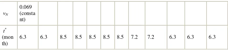
Inputs and parameter values are summarized in Table 1, while outputs are presented in Fig. 2 and
Fig. 3. The computed runoff follows the observed series fairly closely having a maximum departure of 11 mm or about 10% in March. Observed runoff has a root-mean-square value of month-by-month departures from its annual average of ±10.1 mm per month; the correlation coefficient for these two series is 0.98. The maximum of the effective mass forcing M (see, Eq. (7)) in March is due to the significant decrease of effective flushing frequency following the precipitation peak (Fig. 2) while the minimum of M coincides with the P-minimum in August.
http://www.sciencedirect.com/science?_ob=ArticleURL&_udi=B6VBS-49JX91S-Monthly means of: (1) inputs, including global radiation G (1928–1941), precipitation P (1866– 1923), and observed runoff Nobs (1976–1978), and, (2) parameter values resulting from the calibration process for evapoclimatonomy of the Region of Jakarta
http://www.sciencedirect.com/science?_ob=ArticleURL&_udi=B6VBS-49JX91S-νN 0.069 (consta
nt)
t*
(mon th)
6.3 6.3 8.5 8.5 8.5 8.5 8.5 7.2 7.2 6.3 6.3 6.3
Full-size image (8K)
Fig. 2. Evapoclimatonomy for Jakarta, years 1928–1941. P=average precipitation (mm per month); P=P−N−E=reduced mass input (mm per month); M = t*P = effective forcing function (mm equivalent); m=exchangeable soil moisture (mm) computed with the aid of the climatonomic transform of M−m=dm/dτ; using parameters as summarized in Table 1.
Full-size image (16K)
Fig. 3. Evapoclimatonomy for Jakarta. Runoff and evapotranspiration generated using parameter values summarized in Table 1. Month-to-month average of observed runoff for period 1976– 1978 is included for comparison.
Lagging considerably behind P, exchangeable soil moisture (m) peaks with 679 mm in April and decreases gradually in the following months to a minimum of 492 mm in November. Both runoff and evapotranspiration follow essentially the precipitation pattern with the exception that the minimum of evapotranspiration occurs in July while precipitation is lowest in August; E
continues to increase until the maximum appears in February when precipitation is highest.
5. Evapoclimatonomy of Krakatau
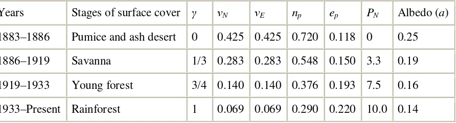
http://www.sciencedirect.com/science?_ob=ArticleURL&_udi=B6VBS-49JX91S-surface albedo, a, for each stage of surface cover can be based on literature values for corresponding ground types (see, for example, [Sellers, 1965] and [Budyko, 1958]; Jackson, 1977). The last column of Table 2 in comparison with albedos for Jakarta shows that from desert to rainforest albedo changes from 0.25 to 0.14. This is significantly larger than the month-to-month variations included in Table 1. It may be assumed that the climatonomic parameters behave in a similar manner. With this assumption, the representative parameters of the rainforest or climax stage on Krakatau will be taken as the annual averages of the calibration results for the Jakarta region summarized in Table 1.
Table 2.
Evapoclimatonomy experiment: assessment of effects of stages of surface cover on Krakatau Island after the 1883 eruption using as auxiliary parameter =Index of Restoration
Years Stages of surface cover νN νE np ep PN Albedo (a)
1883–1886 Pumice and ash desert 0 0.425 0.425 0.720 0.118 0 0.25
1886–1919 Savanna 1/3 0.283 0.283 0.548 0.150 3.3 0.19
1919–1933 Young forest 3/4 0.140 0.140 0.376 0.193 7.5 0.16
1933–Present Rainforest 1 0.069 0.069 0.290 0.220 10.0 0.14
The parameters for the extreme anomaly on Krakatau can only be estimated with reference to analysis results obtained for similar non-vegetated active surface; the possible range of estimates is furthermore restrained by certain physical limiting conditions. Estimates for the transient stages are interpolated between extreme anomaly and climax with the aid of an auxiliary ratio
called “Index of Restoration” which is =0 for the extreme anomaly of pumice and ash desert, and gradually changes to =1 for rainforest climax.
Let p denote any climatonomic parameter which has the anomalous value p=A if =0, and changes to the climax value of p=C if =1. A simple interpolation formula for 0≤ ≤1 which satisfies these boundary conditions is
(11)
By writing A=C+(1+C)/n where n is a suitably chosen integer the interpolation formula can be
reformulated in terms of C, γ and n instead of A, as
http://www.sciencedirect.com/science?_ob=ArticleURL&_udi=B6VBS-49JX91S-Let us begin with estimates for the parameters of immediate depletion. Least important is the threshold value PN since climax value with PN=10 mm per month is small in comparison with precipitation of the driest month. The extreme anomaly may have zero value for the threshold; for consistency, let PN=10 . The immediate runoff ratio has a representative climax value of
np=0.29. Since forest reduces runoff (see, for example, Jackson, 1977) np is low on surface with forest. Hence, for the desert stage 0.29<np<1. A value estimated by Molion (1975) for deforestation in Amazon basin is the case when n=3 in the above formula, which gives
np=(2.16− )/(3+ ), i.e. np=0.72 for extreme anomaly. The immediate evaporivity has a representative climax value of ep=0.22. Normally, immediate evaporivity is larger when more water is available on the surface, i.e. when immediate runoff is small. Also, interception of rain by vegetation increases ep. Therefore, the extreme anomaly will be a smaller positive value, i.e. 0<ep<0.22. Tentatively, ep=0.12 is adopted for the desert stage which suggests n=−12 to give
ep=(1.42+ )/(12− ).
Consistent with climax conditions, νN is assumed to equal νE for all stages. As a consequence of this assumption , recalling that t*=1/(νN+νE). Thus, it is sufficient to deal with estimates of t* only. The rainforest value of νN=0.069 corresponds to t*=7.25 months. According to Geiger (1971), forest floor has a high water-absorption capacity and releases water more slowly than other soil. This suggests relatively low values of t* for the extreme anomaly, as well as the transitional stages. According to Lettau (personal communication) the climatonomical
interpretation of Köppen’s criterion (Köppen, 1936) for the demarcation between the tropical
rainy climates of rainforest (Köppen’s climate class Am) and savanna (Köppen’s climate class Aw) suggests that for savanna t*<1.91 months. Because 1 month is the selected basic time increment for the annual cycle analysis, a restraint for t* on the lower side of a possible range is t*=1
month; namely, if t*<1 month it would not be realistic to separate immediate from delayed depletion processes. This suggests the following range for the retention time of soil moisture:
1 month<t*(desert)<t*(savanna)<1.91 month
The range may be narrowed by assuming that t* (desert) is closer to 1 month than to 2.1 month which suggests to write 1 month<t* (desert) < 1.45 month, or in terms of respondances, for desert stages: 0.69<νN+νE<1.00. The above establishment range of ν values is produced by Eq.
http://www.sciencedirect.com/science?_ob=ArticleURL&_udi=B6VBS-49JX91S-Full-size image (4K)
Fig. 4. Diagram of successions on Krakatau since 1883 until 1933; B: beach vegetation, C: Cyanophyceae (blue-green algae), F: ferns, G: grass, T: trees.
Large immediate runoff and small immediate evaporation are characteristics of the extreme anomaly of pumice and ash desert. The runoff ratio is high, C*=0.85, and could be even higher considering the fact that the np parameter of 0.720 might be an under-estimate for bare rocks. Of primary importance for the pioneers of vegetation are soil moisture and lowering of surface temperature through evaporative cooling. The variation of m and E for the four stages of surface cover is illustrated in Fig. 5.
Full-size image (10K)
Fig. 5. Annual cycle of exchangeable soil moisture (mm water column) and evapotranspiration (W/m2) on Krakatau; modelled as representative area average using climatonomic parameters before eruption and for the three stages of restoring the tropical rainforest.
http://www.sciencedirect.com/science?_ob=ArticleURL&_udi=B6VBS-49JX91S-(personal communication) satisfies Köppen’s criterion for the tropical climate Aw accompanied by savanna. Inland vegetation no longer consisted mainly of ferns in 1897, instead a dense growth of grasses were forming savanna. Closed plant communities began to appear. Evapotranspiration minimum was already twice as large in comparison with the desert extreme, with a maximum of 59 mm month in February. It is very regrettable that no quantitative records on surface or air temperatures were made. A visit by Backer in 1908 (see Docters van Leeuwen, 1936) revealed that a narrow strip of mixed woodland characteristic of the rainforest of Java had already grown behind the beach vegetation; above this mixed forest the grass still predominated while ferns persisted above 400 m altitude. When the next investigation was made in 1919 the mixed woodland first noted in 1908 had developed and extended. Evapotranspiration was almost back to normal in the young forest phase with an average of 54 mm per month; this was due to the significant decrease in the runoff ratio from 0.76 in the savanna to 0.67 in the young forest. The retention-time parameter of soil moisture for the rainforest climax was t*=7.25 month which was double the value obtained for the young forest.
The numerical modelling of annual cycles of the soil moisture for the four characteristic stages
during the first half century of Krakatau’s recolonization has been compared with taking four “snapshots” of the continuous ecological development. Each of these “snapshots” produces the
picture of a characteristic climatic annual cycle for each stage of vegetation succession process. Technically, the climatonomic transform permits numerical forward integration with gradually changing parameter values, beginning in the present problem with the extreme anomaly at its perhaps settled state about early 1884, and ending with the end of 1933, or after vegetation succession climax was reached as soon as information on parameter values and possible feedbacks by the development of a vegetation cover are more securely established.
6. Conclusion
Evapoclimatonomic parameterization and modelling techniques were used to reconstruct climatic water budget status on Krakatau Island for the four stages of surface cover during the 50 years following the 1883 eruption. Assuming unchanged macroclimatic inputs of precipitation and insolation, soil water balances were analyzed and annual cycles of soil moisture were computed. The parameters for the extreme anomaly were estimated based on lower and upper
bound values. Specifically, there were six parameters estimated, namely, partial “flushing frequency” due to evaporative depletion of exchangeable soil moisture (νE), partial “flushing
frequency” due to subsurface depletion of exchangeable soil moisture (νN), immediate runoff ratio (Np), immediate evaporivity (ep), threshold value of precipitation (PN) and local surface albedo (a). These estimations required a number of tentative assumptions; significant improvements can be expected only when more reliable data on hydrology and micro to meso meteorology are available.
The drastic change in surface cover from rainforest to pumice–ash desert produced a significant lowering of soil moisture contents. The most important effect of the resulting reduction in evaporative cooling was a substantial increase in temperature. Although immediate depletion of the abundant rainfall (about 2 m per year) was large, not all runoff might have left the island. A
http://www.sciencedirect.com/science?_ob=ArticleURL&_udi=B6VBS-49JX91S-localities. The importance of evaporative cooling from zero evaporation in the first phase (pumice–ash desert) to a moderate evaporation (36 mm per month) in the second phase (savanna) must have brought significant reduction of maximum surface temperature which, according to
Mayer and Poljakoff-Mayber (1975), is from above to below the germination threshold. Provided all of the essential plant nutrients were sufficiently available, surface depressions in the lava rocks filled initially with dry ashes and after a few wet seasons with water-soaked ashes, very likely offered relatively favourable conditions for seed germination since any local accumulation of rain water must have intensified evaporative cooling. After three or more wet monsoon
seasons a “water table” below the ash and pumice layers might have locally built up to a level which caused an increase in retention time so that t* began to reach values characteristic of the savanna type of tropical vegetation.
The annual total of precipitation as well as precipitation of the driest month was always corresponding to Köppen’s climate class Af (tropical rainforest with Pmin=60 mm per month)
which produces rainforest despite the fact that Krakatau’s savanna stage lasted for more than
three decades. It can be concluded that the gradual increase of t* needed nearly 50 years to arrive at the high-retention time of more than 5 months demanded by the tropical rainforest vegetation.
References
Albrecht, 1940 Albrecht, F., 1940. Untersuchugen über den Warmehaushalt der Erdoberfläche in verschiedenen Klimagebieten. Wissenschaftliche Abhandlungen Band VIII, No. 2. Julius Springer, Berlin, pp. 63–71.
Backer, 1929 Backer, C.A., 1929. The problem of Krakatoa as seen by a botanist. Weltevreden, Java, 299 pp.
Baumgartner et al., 1976 A. Baumgartner, H. Mayer and W. Metz, Globale Verteilung der Oberflächenalbedo, Meteorologische Rundschau 29 (1976), pp. 38–43.
Bey, 1997 Bey, A., 1997. Development of Climatic Water Balance Model for a Region with Defined Boundaries. Paper Presented in the First National Joint Seminar on Environment, Jakarta 1997. Osaka Gas Foundation, Osaka, 12 pp.
Boerema, 1930 Boerema, J., 1930. Results of Meteorological Observation at Batavia 1866–1925. Batavia, pp. 80–118.
Boerema and Berlage, 1948 Boerema, J., Berlage Jr., H.P., 1948. Solar Radiation Measurements in the Netherlands Indies. Verhandelingen No. 34. Soerabaja, 48 pp.
Braak, 1925 C. Braak, Het Klimaat van Nederlandsch-Indië. Koninklijk Magnetisch en Meteorologisch Observatorium te Batavia, Verhandelingen 8 (1) (1925), p. 800.
Budyko, 1958 Budyko, M.I., 1958. In: Stepanova, N.A. (Trans.), Heat Balance of the Earth’s
Surface (Teplovoi balans zemnoi poverkhnosti, 1956). U.S. Weather Bureau, Washington, D.C., 25 pp.
Docters van Leeuwen, 1936 Docters van Leeuwen, W.M., 1936. Krakatau, 1883 to 1933. A. Botany. Annales du Jardin Botanique de Buitenzorg, vol. XLVI–XLVII. Leiden, 506 pp.
Ernst, 1908 Ernst, A., 1908. The New Flora of the Volcanic Island of Krakatau. Cambridge Press, Cambridge, 74 pp.
http://www.sciencedirect.com/science?_ob=ArticleURL&_udi=B6VBS-49JX91S-Jackson, 1977 Jackson, I.J., 1977. Climate, Water and Agriculture in the Tropics. Longman Inc., NY, 248 pp.
Kaimuddin, 2000 Kaimuddin, 2000. Dampak Perubahan Iklim dan Tataguna Lahan terhadap Neraca Air Das di Sulawesi Selatan. Ph.D Theses. Post Graduate Program, Bogor Agricultural University, Bogor.
Kondratyev, 1969 Kondratyev, K.Ya., 1969. Radiation in the atmosphere. International Geophysics Series, vol. 12. Academic Press, NY, 912 pp.
Koppen, 1936 Köppen, W., 1936. Das Geographische System der Klimate. Handbuch der Klimatologie. Berlin, 283 pp.
Lettau, 1969 H. Lettau, Evapotranspiration climatonomy I: a new approach to numerical prediction of monthly evapotranspiration, runoff, and soil moisture storage, Mon. Wea. Rev. 97 (1969), pp. 691–699. Full Text via CrossRef
Lettau and Baradas, 1973 H.H. Lettau and M.W. Baradas, Evapotranspiration climatonomy II: refinement of parameterization, exemplified by application to the Mabacan river watershed,
Mon. Wea. Rev. 101 (1973), pp. 636–649. Full Text via CrossRef
Lettau and Lettau, 1975 Lettau, H., Lettau, K., 1975. Regional climatonomy of tundra and boreal forests in Canada. In: Climate of the Arctic. Proceedings of the 17th AAAS Alaskan Science Conference. Fairbanks, Alaska, pp. 209–221.
Mayer and Poljakoff-Mayber, 1975 Mayer, A.M., Poljakoff-Mayber, A., 1975. The Germination of Seeds. Pergamon Press Ltd., Oxford, England, 92 pp.
Mohr, 1944 Mohr, E.C.J., 1944. In: Pendleton R.L. (Trans.), The Soil of Equatorial Regions with Special Reference to the Netherlands East Indies. Ann Arbor, Michigan, 766 pp.
Molion, 1975 Molion, L.C.B., 1975. A Climatonomic Study of the Energy and Moisture Fluxes of the Amazonas Basin with Consideration of Deforestation Effects. University of Wisconsin, Madison, 133 pp.
Oguntoyinbo, 1970 J.S. Oguntoyinbo, Reflection coefficient of natural vegetation, crops, and urban surfaces in Nigeria, Quart. J. Roy. Met. Soc. 96 (1970), pp. 430–441. Full Text via CrossRef
Oke, 1978 Oke, T.R., 1978. Boundary Layer Climates. Methuen & Co., Ltd., London, 372 pp.
Richards, 1964 Richards, P.W., 1964. The Tropical Rain Forest. An Ecological Study. Cambridge University Press, 450 pp.
Ridley, 1930 Ridley, H.N., 1930. The Dispersal of Plants Throughout the World. L. Reeve & Co., Ltd., Kent, 744 pp.
Sellers, 1965 Sellers, W.D., 1965. Physical Climatology. The University of Chicago Press, Chicago, 272 pp.
Supornrutana, 1971 Supornrutana, S., 1971. Climatonomy of Bangkok. Department of Meteorology, University of Wisconsin, Madison, 49 pp.
Symons, 1888 Symons, G.J., 1888. The eruption of Krakatoa, and subsequent phenomena. Report of the Krakatoa Committee of the Royal Society. Trübner & Co., London, 494 pp.
Treub, 1888 M. Treub, Notice sur lanouvelle flore de Krakatau, Ann. Jard. Bot. Buitenz. 7 (1888), pp. 213–223.
Verbeek, 1885 Verbeek, R.D.M., 1885. Krakatau. Batavia, 164 pp.