Statistical models for small area estimatoin

(1)

(2)

ix

Inventory Model With Gamma Distribution

Hadi Sumadibrata, Ismail

Bin Mohd

642

Accuracy Analysis Of Naive Bayesian

Anti-Spam Filter

Ruslam, Armin Lawi, And

Sri Astuti Thamrin

649

A New Method For Generating Fuzzy Rules From Training Data

And Its Application In Financial Problems

Agus Maman Abadi,

Subanar, Widodo, Samsubar

Saleh

655

The Application Of Laws Of Large Numbers In Convergence

Concept In Probability And Distribution

Georgina M. Tinungki

662

An Empirical Bayes Approach for Binary Response Data in

Small Area Estimation

Dian Handayani, Noor

Akma Ibrahim, Khairil A.

Notodiputro, MOhd. Bakri

Adam

669

Statistical Models For Small Area Estimation

Khairil A Notodiputro,

Anang Kurnia, and Kusman

Sadik

677

Maximum Likelihood Estimation For The Non-Separable Spatial

Unilateral Autoregressive Model

Norhashidah Awang,

Mahendran Shitan

685

Small Area Estimation Using Natural Exponential Families With

Quadratic Variance Function (Nef-Qvf) For Binary Data

Kismiantini

691

Using An Extended And Ensemble Kalman Filter Algorithm For

The Training Of Feedforward Neural Network In Time Series

Forecasting

Zaqiatud Darojah, M. Isa

Irawan, And Erna Apriliani

696

Estimation Of Outstanding Claims Liability And Sensitivity

Analysis: Probabilistic Trend Family (PTF) Model

Arif Herlambang, Dumaria

R Tampubolon

704

Expected Value Of Shot Noise Processes

Suyono

711

Modelling Malaysian Wind Speed Data Via Two Paramaters

Weibull

Nur Arina Basilah Kamisan,

Yong Zulina Zubairi, Abdul

Ghapor Hussin, Mohd.

Sahar Yahya

718

Application Of Latin Hypercube Sampling And Monte Carlo

Simulation Methods: Case Study The Reliability Of Stress

Intensity Factor And Energy Release Rate Of Indonesian

Hardwoods

Yosafat Aji Pranata And

Pricillia Sofyan Tanuwijaya

726

The Development Of Markov Chain Monte Carlo (Mcmc)

Algorithm For Autologistic Regression Parameters Estimation

Suci Astutik, Rahma

Fitriani, Umu Sa’adah, And

Agustin Iskandar

734

A Note About Dh-Fever Estimation With ARIMAX Models

Elly Ana, Dwi Atmono

Agus W

741

Evaluation Of Additive-Innovational Outlier Identification

Procedure For Some Bilinear Models

I

smail, M.I., Mohamed, I.B.,

Yahya, M.S.

(3)

xi

Model By Spectral Regression Methods

Iriawan, Suhartono

Application Of Cluster Analysis To Developing Core Collection

In Plant Genetic Resources

Sutoro

875

Small Area Estimation With Time And Area Effects Using A

Dynamic Linear Model

Kusman Sadik And Khairil

Anwar Notodiputro

880

Statistical Analysis Of Wind Direction Data

Ahmad Mahir Razali, Arfah

Ahmad, Azami Zaharim

And Kamaruzzaman Sopian

886

Generalized Additive Mixed Models in Small Area Estimation

Anang Kurnia, Khairil A.

Notodiputro, Asep

Saefuddin, I Wayan

Mangku

891

Kernel Principal Component Analysis In Data Visualization

Ismail Djakaria, Suryo

Guritno, Sri Haryatmi

898

GARCH Models And The Simulations

Nelson Nainggolan, Budi

Nurani Ruchjana And

Sutawanir Darwis

906

Rainfall Prediction Using Bayesian Network

Hera Faizal Rachmat, Aji

Hamim Wigena, and Erfiani

911

Identifying Item Bias Using The Simple Volume Indices And

Multidimensional Item Response Theory Likelihood Ratio

(Irt-Lr) Test

Heri Retnawati

916

Ordinary Kriging And Inverse Distance Weighting For Mapping

Soil Phosphorus In Paddy Field

Mohammad Masjkur,

Muhammad Nuraidi and

Chichi Noviant

924

K-Means Clustering Visualization

On Agriculture Potential Data

For Villages In Bogor Using Mapserver

Imas S. Sitanggang, Henri

Harianja, and Lailan

Syaufina

932

Some Methods To Estimate The Number Of Components In A

Mixture

M. A. Satyawan, A. H.

Wigena, Erfiani

941

A Probabilistic Model For Finding A Repeat

Triplet Region In DNA Sequence

Tigor Nauli

947

Application Of Spherical Harmonics In Determination Of Tec

Using Gps Observable

Mardina Abdullah, Siti

Aminah Bahari, Baharudin

Yatim, Azami Zaharim,

Ahmad Mahir Razali

954

Testing Structure Correlation Of Global Market By Statistic Vvsv Erna Tri Herdiani, and

Maman A. Djauhari

961

Exploring the MAUP from a spatial perspective

Gandhi Pawitan

967

Estimation of RCA(1) Model using EF:

A new procedure and its robustness

1Norli Anida Abdullah,

2Ibrahim Mohamed,

3Shelton Peiris

996

Second Order Linear Elliptic Operators

In The Unit Square

(4)

xii

POSTER

Study Of Fractional Factorial Split-Plot Experiment

Sri Winarni, Budi Susetyo,

and Bagus Sartono

1012

Improving Model Performance For Predicting Poverty Village

Category Using Neighborhood Information In Bogor

Bagus Sartono, Utami Dyah

S, and Zulhelmi Thaib

1019

Ammi Models On Count Data: Log-Bilinear Models

Alfian Futuhul Hadi

H. Ahmad Ansori Mattjik

I Made Sumertajaya

Halimatus Sa’diyah

1026

Prediction Of Oil Production Using Non Linear Regression By

Sdpro Software

(Special Program Package)

*)

Budi Nurani R , and

Kartlos J. Kachiashvili

1038

An Implementation Of Spatial Data Mining

Using Spatial Autoregressive (Sar) Model

For Education Quality Mapping At West Java

*)

Atje Setiawan A. ,

Retantyo Wardoyo , Sri

Hartati , and Agus Harjoko

1045

Validation Of Training Model

For Robust Tests Of Spread

Teh Sin Yin, and Abdul

Rahman Othman

1056

Spectral Approach For Time Series Analysis

Kusman Sadik

1063

The ACE Algorithm for Optimal Transformations in Multiple

Regression

Kusman Sadik

1066

The Relation Between The Students’ Interaction And The

Construction Of Mathematical Knowledge

Rini Setianingsih

1069

Application of Auto Logistic Regression Spatial Model using

Variogram Based Weighting Matrix to Predict Poverty Village

Introduction

Small Area Estimation (SAE) is an important concept in survey sampling especially for indirect parameter estimation of relatively small samples. This method can be used to estimate parameters of sub population (a domain which is smaller than population). Direct estimation for sub population fails to provide enough precision since the sample size is small.

Another method which can be used to obtain higher precision in small area estimation may be developed by linking some information in particular area with some other areas through appropriate model. This procedure is called indirect estimation. The procedure involves data from other domains. In other words, small area estimation model is borrowing strength from sample observation of related areas through auxiliary data (recent census and current administrative records) to increase effective sample size (Rao, 2003).

In this paper we will discuss small area estimation through indirect method or estimation based models. One of the problems found in using this procedure is low precision of linear model for modeling of auxiliary data. In this paper we propose a class of generalized additive mixed model to improve the model of auxiliary data in small area estimation. Moreover since some surveys are carried out periodically so that the estimation could be improved by incorporating both the area and time random effects we also proposed a state space model which accounts for the two random effects.

2.

Brief review of related topics

2.1 Small area estimation based on linear mixed model

There are essentially two-types of models in small area estimation. The first is area level model that relate small area direct estimator to area-specific auxiliary data xi = (x1i, x2i, …, xpi). We assume the

parameter of interest θi = xi’β + υi where υi ~ N(0, A) and direct estimator θˆi= θi + ei where ei|θi ~ N(0,

Di) and Di known. The model combines the parameter of interest and the indirect estimates forms θˆi = xi’β + υi + ei which is a case of generalized linear mixed model. The second is unit level model. In this The 3rd

(6)

678

model the information is available at the sampling unit level and modeling is done based on individual data xij = (x1ij, x2ij, …, xpij) and we have model yij = xijTβ + υi + ei that is a more complex model.

We consider the following Fay-Herriot model (see Fay and Herriot, 1979) for the basic area level model

yi = xi’β + υi + ei

where υi and ei are independent with υi ~ N(0, A) and ei ~ N(0, Di) for i = 1, 2, ..., k. We assume that

β and A unknown but Di (i = 1, 2, ..., k) are known.

The best predictor (BP) of θi = xi’β + υi if β and A known is given by

i

θˆBP = θˆ_i(yi|β, A) = xi’β + (1 – Bi)(yi - xi’β)

where Bi = Di/(A + Di) for i = 1, 2, ..., k. Let θˆ_i BP

= θˆ_i_(y_i_|β_{, A) is also Bayes estimator of}θ_i_{under the} following Bayesian models:

(i) yi|θi ~ N(θi, Di)

(ii) θi ~ N(xi’β, A) is prior distribution for θi , i = 1, 2, ..., k.

The Bayes estimator is given from the posterior distribution

(θi|yi, β, A) ~ N

(

_A

)

_D1 _A1 -1

)

' x D y

)

+

(

,

+

i i i i β

= N

(

)

i i

i A+D

AD i i D + AA

i' + (y - x ' ),

x β β

It follows that

i θˆEB

= E(θi|yi, β, A) = xi’β + (1 – Bi)(yi - xi’β)

where MSE(θˆ_iEB

) = Var(θi|yi, β, A) =

i i D + A AD

= (1 – Bi)Di = g1i(A). The estimator θˆ_iBP is equivalent

with θˆ_iEB for normally distributed cases.

When A is known, β could be estimated using the weighted maximum likelihood method

log L(β, V) = -

2

1

log|V| -

2

1

(Y - Xβ)’ V-1(Y - Xβ)

where V = Diag(A + D1, A + D2, ..., A + Dk).

Let β* = βˆ_i(A) = (X’V-1X)-1 X’V-1Y and by replacing β with β* in the θˆ_iBP, we get the best linear unbiased predictor (BLUP) of θi given by

i θˆBLUP

= θˆ_i_(y_i_{|A) = x}_i_’β_{* + (1 – B}_i_)(y_i_{- x}_i_’β_*)

Ghosh and Rao (1994) describe the MSE(θˆ_iBLUP

) = g1i(A) + g2i(A), where

g1i(A) =

i i D + A AD

= (1 – Bi)Di, and

g2i(A) = Di

2

/(A + Di) [xi’(X’V -1

X)-1 xi]

= Di (1 – Bi) [xi’(X’V-1X)-1 xi] untuk i = 1, 2, …, k.

However, in practice both β and A is unknown. To estimate A, we can use maximum likelihood

(ML), restricted/residual maximum likelihood (REML) or method of moment (MM). If we replace β by

β

ˆ and A byAˆ in the BLUP (θˆ_iBLUP) estimator, we get the empirical best linear unbiased predictor (EBLUP)

i

θˆEBLUP = θˆ_i(yi|Aˆ) = xi’βˆ + (1 – Bˆi)(yi - xi’βˆ)

If defined MSE of θˆ_iEBLUP

is MSE(θˆ_iEBLUP

) = E(θˆ_iEBLUP

- θi)2 = Var(θˆ_iEBLUP) + (Bias θˆ_iEBLUP)2,

Kacker and Harville (1984) reformulated it as

(7)

679

where H1i(A) = MSE(θˆ_i BLUP

) = g1i(A) + g2i(A) and H2i(A) = E(θˆ_i EBLUP

- θˆ_iBLUP)2. Leading term g1i(A)

lead to large reduction in MSE relative to the MSE of the direct estimator, g2i(A) is due to estimating of β

and H2i(A) is due to estimating A.

Prasad and Rao (1990) used the Taylor series method to estimate g1i(A), g2i(A) and H2i(A). The MSE

estimator of θˆ_i

MSE(θˆ_iEBLUP)PR = g1i(ˆA) + g2i(Aˆ) + 2 g3i(Aˆ)

where g3i(Aˆ) = ∑k

1 = j

2 j 3 i 2

2

i _(A₊_D ₎

) D + (A k

2D _{. The MSE(}

i

θˆ₎PR_{is identical to the Bayes risk as defined by Butar}

and Lahiri (2001).

2.2 Generalized additive (mixed) model

Multiple regression analysis is one of the most widely used statistical techniques. It is a powerful tool when its assumptions are met, including that the relationships between the predictors and the response are well described with a defined function (e.g., straight-line, polynomial, or exponential). In many applications, however, the reliance on a defined function is limited. Many phenomena do not have a relationship that can be easily defined.

To overcome the above difficulties, Stone (1985) proposed the additive model to solve them. These models estimate an additive approximation to the multivariate regression function. The advantages of this approximation are at least twofold. First, since each of the individual additive terms is estimated using a univariate smoother, the curse of dimensionality is avoided, at the cost of not being able to approximate universally. Second, estimates of the individual terms explain how the dependent variable changes with the corresponding independent variables.

In general, generalized additive models (GAM) enable us to relax this assumption by replacing a defined function with a non-parametric smoother to uncover existing relationships. Smoothing is a method that will highlight a trend by separating it from variability due to noise. Several different smoothers are available, but the most commonly used are spline or loess. Smoothers have a parameter that can be used to control the closeness of the fit of the trend to the data. For detail about GAM please refer to Hastie and Tibshirani (1990).

GAM is additive models since they simultaneously fit the distinct effects of each independent variable. Each effect can be estimated using either a smoother or a defined function, leading to the description of GAM as semi parametric. GAM is appropriate under the assumption of the absence of interaction effects.

GAM also offers the added flexibility of permitting non-normal error distributions. This allows modeling response variables with distributions such as binomial and Poisson. Generalized Additive Mixed Models (GAMM) has also been recently developed to incorporate random effects, which are an additive extension of Generalized Linear Mixed Model (GLMM) in the spirit of Hastie and Tibshirani (1990).

Let Y be a response random variable and X1, X2, ... , Xp be a set of predictor variables. A regression procedure can be viewed as a method for estimating the expected value of Y given the values of X1, X2, ... , Xp. The standard linear regression model assumes a linear form for the conditional expectation

E(Y | X1, X2, …, Xp) = β0 + β1X1 + β2X2 + … + βpXp

Given a sample, estimates of β0, β1, β2, …, βp are usually obtained by the least squares method. The

additive model generalizes the linear model by modeling the conditional expectation as

E(Y | X1, X2, …, Xp) = s0 + s1(X1) + s2(X2) + … + sp(Xp)

where si(X), i = 1,2, ... , p are smooth functions.

(8)

680

Generalized additive models address these difficulties, extending additive models to many other distributions besides just the normal. Thus, generalized additive models can be applied to a much wider range of data analysis problems. Similar to generalized linear models, generalized additive models consist of a random component, an additive component, and a link function relating the two components. The response Y, the random component, is assumed to have exponential family density. The mean of the response variable µ is related to the set of covariates X1, X2, ... , Xp by a link function g. The quantity

( )

o i i

= s + s X

η

Σ

defines the additive component, where s1(·), ... , sp(·) are smooth functions, and the relationship between µ and η is defined by g(µ) = η. The most commonly used link function is the canonical link, for which η = θ.

Furthermore, Lin and Zhang (1999) proposed Generalized Additive Mixed Models (GAMM) for over dispersed and correlated data. They explored the Generalized Linear Mixed Model (GLMM) representation of the smoothing spline estimators and estimated the smoothing parameter using REML. Following Breslow and Clayton (1993), Lin and Zhang (1999) used Double Penalized Quasi-Likelihood to estimate beta and REML is used to estimate the variance components.

3.

The GAMM approach for small area estimation

Rao (2003) provided extensive review of the most commonly used estimators, including synthetic and composite estimator, empirical best unbiased linear predictors, empirical Bayes and hierarchical Bayes approach. These estimators are based on parametric approach. We propose a class of nonparametric approach, generalized additive mixed model (GAMM). The GAMM approach has significant advantages over its parametric approach to model auxiliary variable. The adoption of this approach in small area estimation is straight forward.

Consider an extension of the Fay-Herriot model for the basic area level model

yi = xi’β + υi + ei , i = 1, 2, ..., k

where β is coefficient regression parameters, υi are random effect area, and ei are sampling errors. Also

assume ei ~ (0, Di), υi ~ (0, A) and that they are independent. Di is usually assumed to be known, see Rao

(2003).

We assume that yi and xi are related by a smooth function m(.). Let X be the random vector of

predictors, thus

yi = m(xi) + υi + ei , i = 1, 2, ..., k

where υi|X ~ (0, υ(xi)), ei ~ (0, Di), and ei and υi are independent. The small area mean functions is

θi(xi) = m(xi) + υi

are linear combination of mean m(xi) and the random effects υi. We can use an estimator of the mean

function using a linear smoother such as smoothing splines, regression splines, and local polynomial regression. For detail discussion of these methods, see Hastie and Tibshirani, (1990).

If we use Kernel smoothing function to estimate m(xi), the best predictor for small area means θi can

be written as

E(θi|yi) = γi yi + (1 - γi) mˆ_h(xi)

where γi = υ(xi) / (υ(xi) + Di). To approximate MSE, we substitute xi’β in linear mixed model with

h mˆ (xi).

mse(θˆ_i_{) =} i u2 2 i u

D

D +

ˆ ˆ

σ σ

+

(

)

2

(

( )

)

h i

1-ˆγ mse mˆ x + 2

(

2

)

-3

( )

2

i u i u

2D ˆσ + D mse ˆσ

4.

Evaluation and application of GAMM

We illustrate the GAMM approach using two data set. The first data was hypothetical data for 32 small area where υi and ei have normal distribution with mean 0 and variance 1. Y, which is the variable

(9)

681

is 0.0193 and the EBLUP estimator is 0.0212. Further, the relative root mean square error (RRMSE) of GAMM approach is 0.0289, while the EBLUP estimator is 0.0327/

The second data set was real data taken from PODES 2005 and SUSENAS 2005 for Bogor Municipality. Both data were collected by BPS (Statistics Indonesia). Y is unemployment level which is indicated as percentage of unemployment from group of “age work” for each village in Bogor Municipality. Percentage of men (X2), percentage of non-permanent housing (X5), percentage of letter poor statement (X7), and percentage of pre prosperous-family and prosperous-family 1 (X8) are used as auxiliary variable.

Table 1. Estimator of Unemployment Level in Bogor Municipality

Village Direct GAMM EBLUP Village Direct GAMM EBLUP

1002 Pamoyanan 13.04 12.64 13.03 4006 Sempur 10.94 10.38 10.93

1005 Kertamaya 8.42 8.86 8.43 4010 Kebonkelapa 12.07 12.06 12.07

1006 Rancamaya 25.00 23.36 24.94 5002 Pasirkuda 20.00 17.60 19.95

1009 Muarasari 1.85 1.97 1.85 5003 Pasirjaya 13.51 12.91 13.49

1013 Batutulis 6.38 6.46 6.39 5004 Gunungbatu 10.64 10.31 10.63

1015 Empang 3.33 3.42 3.34 5006 Menteng 10.91 10.91 10.90

1016 Cikaret 9.80 9.74 9.80 5008 Cilendek Barat 16.67 15.81 16.64

2002 Sindangrasa 1.67 1.75 1.67 5009 Sindangbarang 6.38 6.72 6.39

2006 Sukasari 8.33 8.21 8.33 5012 Situgede 4.00 4.24 4.00

3001 Bantarjati 5.45 5.56 5.46 5015 Curugmekar 10.42 10.25 10.41

3002 Tegalgundil 6.90 6.98 6.90 6001 Kedungwaringin 6.38 6.33 6.39

3004 Cimahpar 3.28 3.59 3.29 6003 Kebonpedes 9.43 9.55 9.44

3006 Cibuluh 10.53 10.91 10.53 6004 Tanahsareal 11.54 10.92 11.53

3007 Kedunghalang 9.09 8.94 9.09 6005 Kedungbadak 6.38 6.35 6.38

3008 Ciparigi 4.88 5.16 4.88 6007 Sukadamai 12.50 11.99 12.49

4002 Gudang 14.81 14.48 14.79 6009 Kayumanis 5.45 5.56 5.47

4004 Tegallega 2.27 2.53 2.28 6011 Kencana 6.25 6.57 6.26

(10)

682

Table 1 exhibits the results from each method to estimate unemployment level in Bogor Municipality. The RRMSE for direct estimator, GAMM approach and EBLUP are 0.0361, 0.0326 and 0.0335. Actually all of the estimators support direct estimator. The possible factors which can affect this condition is variance between small area that was higher than variance sampling error within small area. However, the GAMM approach was able to reduce the auxiliary variable influence which was not linear. Figure 1 shows the scatter plot of auxiliary variable while X2 and X7 have not linearity between the auxiliary and the response interest.

It is shown in our study that generalized additive mixed model outperforms generalized linear mixed model in EBLUP at least in two aspects. First, generalized additive mixed model relaxes the assumption of linearity between the predictors and the response and avoids the problem of model misspecification that often happened in EBLUP. Secondly, by incorporating nonlinear effects, generalized additive mixed model helps to discover the hidden pattern of predictors and therefore improves the predictive performance.

5.

State space models

Many sample surveys are repeated in time with partial replacement of the sample elements. For such repeated surveys considerable gain in efficiency can be achieved by borrowing strength across both small areas and time. Their model consist of a sampling error model

=

θ

ˆ

it θit + eit, t = 1, …, T; i = 1, …, m θit = zit

T_β it

where the coefficients βit = (βit0, βit1, …, βitp)T are allowed to vary cross-sectionally and over time, and

the sampling errors eit for each area i are assumed to be serially uncorrelated with mean 0 and variance ψit. The variation of βit over time is specified by the following model:

p

j

v

itj ij j t i j ij itj

,...,

1

,

0

,

0

1

β

, 1,

=













+













=













−

T

It is a special case of the general state-space model which may be expressed in the form

yt = Ztαt + εt; E(εt) = 0, E(εtεt T

) = Σt αt = Htαt-1 + Aηt; E(ηt) = 0, E(ηtηtT) = Γ

where εt and ηt are uncorrelated contemporaneously and over time. The first equation is known as the measurement equation, and the the second equation is known as the transition equation. This model is a special case of the general linear mixed model but the state-space form permits updating of the estimates over time, using the Kalman filter equations, and smoothing past estimates as new data becomes available, using an appropriate smoothing algoritm.

The vector αt is known as the state vector. Let

α

t-1

~

_{be the BLUP estimator of}_α

t-1 based on all

observed up to time (t-1), so that

α

~

_t_|_t_-1= H

α

~

_t_-1is the BLUP of αt at time (t-1). Further, Pt|t-1 = HPt-1HT +

AΓAT is the covariance matrix of the prediction errors

α

~

_t_|_t_-1- αt, where

Pt-1 = E(

α

t-1

~

_-_α

t-1)(

α

t-1

~

_-_α

t-1)T

is the covariance matrix of the prediction errors at time (t-1). At time t, the predictor of αt and its

covariance matrix are updated using the new data (yt, Zt). We have

yt - Zt

α

t|t-1

~

₌_Z

t(αt -

α

t|t-1

~

_{) +}_ε

t

which has the linear mixed model form with y = yt - Zt

α

t|t-1

~

_,_Z₌_Z

t, v = αt -

α

t|t-1

~

_,_G₌_P

t|t-1 and V = Ft,

where Ft = ZtPt|t-1Zt T

+ Σt. Therefore, the BLUP estimator

~

v

= GZ

T

V-1y reduces to

-1 t

α

~

₌ -1 t | t

α

~

₊_P_t|t-1_Z_tT_F_t-1₍_y_t_-_Z_t

-1 t | t

α

~

₎

6.

Application of state space models

(11)

683

[image:11.595.117.471.158.619.2]

and Social Survey, BPS 2003-2005) to demonstrate the performance of EBLUP resulted from state space models .

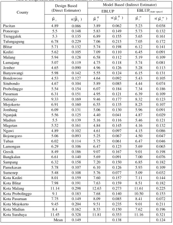
Table 2. Design Based and Model Based Estimates of County Means and Estimated Standard Error

County

Design Based (Direct Estimator)

Model Based (Indirect Estimator)

EBLUP EBLUP(state space)

i

µˆ s(

µ

ˆ

_i) µˆHi s(

H i

µˆ ) ss

i

µˆ s( ss

i µˆ )

Pacitan 4.89 0.086 3.89 0.062 5.23 0.038

Ponorogo 5.5 0.148 5.83 0.149 5.73 0.132

Trenggalek 5.3 0.135 6.89 0.155 5.65 0.161

Tulungagung 6.78 0.229 7.06 0.215 7.05 0.172

Blitar 5.71 0.132 5.74 0.198 6.12 0.141

Kediri 5.62 0.105 7.09 0.110 6.45 0.091

Malang 5.94 0.128 6.58 0.112 5.19 0.109

Lumajang 5.07 0.119 4.75 0.118 5.74 0.081

Jember 4.65 0.090 4.96 0.126 5.28 0.113

Banyuwangi 5.98 0.142 5.55 0.124 6.15 0.131

Bondowoso 4.53 0.127 4.64 0.092 5.43 0.105

Situbondo 4.67 0.104 5.89 0.085 4.44 0.074

Probolinggo 5.54 0.154 6.07 0.184 7.34 0.186

Pasuruan 6.31 0.151 4.95 0.121 6.39 0.109

Sidoarjo 9.33 0.169 9.46 0.177 8.32 0.123

Mojokerto 6.91 0.160 6.55 0.135 8.25 0.107

Jombang 6.09 0.131 5.06 0.130 5.96 0.091

Nganjuk 5.56 0.125 4.40 0.041 4.87 0.029

Madiun 5.5 0.139 5.16 0.116 5.46 0.121

Magetan 5.52 0.161 4.84 0.145 4.16 0.132

Ngawi 4.89 0.102 4.61 0.097 4.15 0.086

Bojonegoro 5.06 0.093 5.25 0.067 4.50 0.047

Tuban 6.02 0.114 5.75 0.061 6.47 0.046

Lamongan 6.29 0.106 6.47 0.123 5.69 0.065

Gresik 8.49 0.186 9.07 0.167 9.01 0.198

Bangkalan 6.61 0.140 5.69 0.091 7.00 0.076

Sampang 6.32 0.158 7.20 0.150 6.85 0.182

Pamekasan 5.78 0.107 6.10 0.126 5.93 0.109

Sumenep 5.48 0.108 5.76 0.077 5.09 0.032

Kota Kediri 8.01 0.159 7.60 0.157 7.11 0.144

Kota Blitar 7.98 0.191 7.63 0.159 8.51 0.182

Kota Malang 11.14 0.298 12.63 0.273 11.61 0.225

Kota Probolinggo 9.1 0.183 7.68 0.140 10.50 0.153

Kota Pasuruan 7.75 0.149 8.09 0.085 8.41 0.072

Kota Mojokerto 9.45 0.204 9.51 0.235 9.01 0.211

Kota Madiun 8.4 0.162 8.33 0.150 7.62 0.196

Kota Surabaya 11.45 0.328 11.81 0.353 11.16 0.321

Mean 0.149 0.138 0.124

Table 2 shows the design based and model based estimates. The design based estimates is direct

estimator based on sampling design. EBLUP estimates, H

i

µˆ , used small area model with area effects (data of Susenas 2005) whereas, EBLUP(ss) estimates, µˆiss, used small area model with area and time

effects (data of Susenas 2003 to 2005). The estimated standard errors are denoted by s(

µ

ˆ

_i), s( H i µˆ ), and

s( ss

i

µˆ ). It is clear from Table 1 that the estimated standard errors of mean for the model based is less than the estimated standard error for the estimates design based. The estimated standard error mean of

EBLUP(ss) is less than EBLUP.

(12)

684

7.

Conclusion

Small area estimation can be used to increase the effective sample size and thus decrease the standard error. The above methods showed that gain in efficiency can be achieved by borrowing strength across small area as well as time. Availability of good auxiliary data and determination of suitable linking models are crucial to the formation of indirect estimators.

8.

Acknowledgements

This work was supported by a research grant from DGHE Ministry of National Education Republic of Indonesia: Development of Small Area Estimation and Its Application for BPS’ Data, Batch IV 2nd years (2007).

9.

References

Butar, F.B. and Lahiri, P. 2001. “On Measure of Uncertainty of Empirical Bayes Small Area Estimator.

Journal of Statistical Planning and Inference.

Breslow, N.E. and Clayton, D.G. 1993. Approximate inference in generalized linear mixed models.

Journal of the American Statistics Association, Vol. 88, pp. 9-25.

Fahrmeir, L. and Lang, S. 2001. Bayesian inference for generalized additive mixed models based on Markov random field priors. Journal of the Applied Statistics, Vol. 50, part 2, pp. 201-220. Fay, R.E. and Herriot, R.A., (1979), “Estimates of income for small places: An application of James-Stein

procedures to Census data”. Journal of the American Statistical Association, Vol. 74, p:269-277 Ghosh, M. and Rao, J.N.K. 1994. “Small Area Estimation: An Appraisal”. Statistical Science, 9, No.1

p:55-93.

Jiang, J. 1996. “REML estimation: Asymptotic behavior and related topics”, Annals of Statistics, 24, :255-286.

Jiang, J., Lahiri, P. and Wan, S.M. 2002. A Unified Jackknife Theory, Annals of Statistics, 30.

Hastie, T. and Tibshirani, R. 1990. Generalized Additive Models. London: Chapman and Hall.

Lin, X and Zhang, D. 1999. Inference in generalized additive mixed models by using smoothing splines.

Journal of the Royal Statistics Society Series B, Vol. 6 part 2, pp. 381-400.

McCulloch, C. 1997. Maximum likelihood algorithms for generalized linear mixed models. Journal of the American Statistics Association, Vol. 92, pp. 162-190.

Prasad, N.G.N. and Rao, J.N.K. 1990. “The Estimation of Mean Squared Errors of Small Area Estimators”. Journal of American Statistical Association, 85, pp. 163-171.

Rao, J.N.K. 1999. Some Recent Advances in Model-Based Small Area Estimation, Survey Methodology,

Vol.25 No.2, pp. 175-186.

Rao, J.N.K. 2003. Small Area Estimation, New York : John Wiley and Sons.

Rao, J.N.K. 2005. Inferential Issues In Small Area Estimation: Some New Developments. Statistics In Transition, December 2005 Vol. 7, No. 3, Pp. 513—526.

Zeger, S.L. and Karim, M.R. 1991. Generalized linear model with random effects: a Gibbs sampling