BUILDING CHANGE DETECTION IN VERY HIGH RESOLUTION SATELLITE
STEREO IMAGE TIME SERIES
J. Tiana,* , R. Qinb, D. Cerraa, P. Reinartza
a
Dept. Photogrammetry and Image Analysis, Remote Sensing Technology Institute, German Aerospace Center (DLR), Germany – (Jiaojiao.tian, Daniele.cerra, Peter.reinartz)@dlr.de
b
Dept. Civil, Environmental and Geodetic Engineering, The Ohio State University, USA- [email protected]
Commission VII, WG VII/5
KEY WORDS: Building, DSM, Change detection, Satellite, Satellite image time series
ABSTRACT:
There is an increasing demand for robust methods on urban sprawl monitoring. The steadily increasing number of high resolution and multi-view sensors allows producing datasets with high temporal and spatial resolution; however, less effort has been dedicated to employ very high resolution (VHR) satellite image time series (SITS) to monitor the changes in buildings with higher accuracy. In addition, these VHR data are often acquired from different sensors. The objective of this research is to propose a robust time-series data analysis method for VHR stereo imagery. Firstly, the spatial-temporal information of the stereo imagery and the Digital Surface Models (DSMs) generated from them are combined, and building probability maps (BPM) are calculated for all acquisition dates. In the second step, an object-based change analysis is performed based on the derivative features of the BPM sets. The change consistence between object-level and pixel-level are checked to remove any outlier pixels. Results are assessed on six pairs of VHR satellite images acquired within a time span of 7 years. The evaluation results have proved the efficiency of the proposed method.
1. INTRODUCTION
Remote sensing data are playing a key role for tracking land cover changes. Along with the improved image data quality and the increased amount of available satellite data in recent years, the details and accuracy of the obtainable information are assumed to be enhanced.
Recent studies have proved the advantages of change analysis based on satellite image time series data (SITS) (Yang and Lo, 2002; Bontemps et al., 2008). However, most of them focus on monitoring changes at a large scale (low resolution) based on stable features, such as vegetation index (Verbesselt et al., 2010; de Jong et al., 2011; Fensholt and Pround, 2012; Chen et al., 2014), to monitor and predict the vegetation evolution. In this work, the increase of spatial resolution and multi-view data capability of satellite sensors are exploited to use SITS for building monitoring at small scales.
To the best of our knowledge, building extraction methods are still under research and there is currently no operationally robust method available. Digital Surface Models (DSMs) have been proved to be very helpful in improving building extraction and change detection accuracy (Tian et al., 2014; Qin and Fang, 2014), as variations in height represent a robust feature to evaluate building changes. However, the quality of the DSMs from satellite stereo imagery depends strongly on the image matching result. If the unmatched region is too large, then it is difficult to interpolate accurate height by using the height information from its neighbourhood. Therefore, building changes may not be detected correctly if they are located within such regions. On the other hand, a direct comparison of multi-sensor stereo imagery introduces many false positive /negatives. Therefore, time-series data could be helpful to improve the quality of each single dataset, as they provide redundant information.
Moreover, comparing images from two dates that are too far apart can not provide detailed information on the progressive construction procedure.
This paper examines the problems and advantages of employing very high resolution (VHR) SITS data for the described purposes. A two-step procedure has been developed: firstly, the quality of single images is improved by using spatial and temporal information. Subsequently, the improved time-series building probability maps are analysed to highlight building changes and identify the type of change which took place at a given building site.
2. DATA DESCRIPTION 2.1 Data description and preprocessing
Table 1. Data Description
No. Satellite Capture date Resolution (m)
PAN MS
These 6 datasets are acquired in different seasons of the year, where the illumination differences and seasonal variations are the major issues for time series change analysis. To eliminate the potential disturbances from these factors, we adopted the approach proposed in Qin et al (2015) to combine the multispectral and height information for extracting the probability of each pixel belonging to buildings.
2.2 Building probability map extraction
Due to the heterogeneity of the images and the influence of the environmental conditions on the spectrum, it is difficult to find a unique index to indicate pixels belonging to buildings across all the available images in the SITS. A feasible way is to use supervised methods to characterize the buildings using a few training samples. Hence Random Forest (RF) (Breiman, 2001) classifier is adopted due to its low computation complexity and good capability of handling large volumes of data. RF provides a probability as the confidence for a given test sample of belonging to a particular class. Following the classic supervised classification paradigm, the probability map extraction is mainly composed of two steps: (1) training sample selection; (2) feature extraction and classification.
2.2.1. Training sample generation
Although the training samples of all the six “DSM+Orthophoto” should be selected separately to ensure correctness, this is a time consuming and tedious process. Rather than extracting a set of samples for each date, we extract then only one sample dataset, and adopt a decision-based method to derive the remaining training samples as shown in Figure 1.
Extracted training
Building Ground & Road Shadow Trees building ground road shadow
add keep delete keep delete
Generated training samples of date B
Figure 1. Flow chart for the generation of training samples.
As shown, the training sample extraction is built on a coarse index-checking procedure. Although we mentioned it is difficult to find indices for urban objects given the varying conditions of the scenes within the time-series, some common indicators can still be used for a coarse estimation. In this procedure, the nDSM (normalized DSM) derived with morphological filtering is used to represent off-terrain objects. MSI (morphological shadow index) and NDVI (normalized difference vegetation index) are used to indicate shadows and vegetation. Although our target is building change detection, multi-class information can be useful to construct distinctive representation of the building class. Moreover, time series change detection can be also applied to classes other than buildings. It should be noted that we only update the samples when there is a large difference between these indicators in the time-series. In figure 1, these differencing threshold in our experiments are taken as T1=1.5,
T2 = 3, and T3 = 0.2.
2.2.2. Feature extraction and classification
There are works proving that combining the spectral and height information for classification can increase the accuracy to a notable level (Huang et al., 2011; Qin et al., 2015). As our intention is to derive the building probability values, pixel-wise classification is used. The following features are extracted for our classification task:
1) Four components after a PCA (Principal Component Analysis) transformation of the multispectral bands;
2) DMP (Differential Morphological Profile) of the panchromatic images;
3) MTHR (Morphological Top-Hat by Reconstruction) of the DSM.
PCA (Jolliffe, 2005) is applied on the multispectral image to capture the spectral information of the feature vector. DMP (Benediktsson et al., 2003) is applied due to its good performance at detecting the spatial structure of images. MTHR is particularly effective to separate off-terrain objects from the ground layer (Qin and Fang, 2014). All the components in the feature vectors are normalized to ensure their equivalent contribution to the classifier. The RF assigns a class label for each pixel, and at the same time gives a confidence value to that pixel, proportional to the probability of that pixel to belong to a particular class.
2.2.3. Refinement of the probability
We define a building probability map (BPM) as the probability of each pixel belonging to the building class. The BPMs across all the dates might not be consistent due to various factors such as the errors in training samples, or classification error due to the highly similar spectral information of different classes, e.g. in the case of heavy snow. Therefore, we perform a consistency refinement on all the BPMs using a bilateral-weighted approach, considering the smoothness of the spatial domain and height discontinuity in the temporal domain:
�(�,�,�) = �−|���
(�,�,�)−��(�,�,�)�||2
2�12 +
−||[�,�]−[�,�]|2 2�22 +
−||���(�,�,�)−���(�,�,�)||2
2�32 (2)
The weight � acts as 3D bilateral-filter that removes the noise on both the spatial directions of each BPM, at the same time being sensitive to height differences. In the refined results, the BPMs with similar height are merged, while BPMs whose heights are significantly different are assigned a small contribution. This is a reasonable consideration, since changes in buildings often bring height differences, in which the BPMs should not be merged. Figure 2 shows a comparison before and after the refinement. The refined BPM shows that buildings are better separated and there are less salt- and pepper noise effects.
Figure 2. BPMs before (a) and after (b) the refinement.
2.3 Building change reference data
The refined BPMs of different dates will be used in our subsequent change detection analysis over the SITS. For the validation purpose, we have manually extracted the per-year building change (YBC) reference map over the test region as shown in Figure 3, where significant building changes occur mainly in 2009, and at the beginning and in the middle of 2011. We sort the single scenes in the SITS according to their acquisition dates. Changes happened in the second date (year 2009) are shown with blue colour. In this test region, no visible building changes occurred from 2009 until the middle of 2010. Orange objects in Figure 3 represent new buildings constructed before January 2011. Changes which took place shortly before May 2011 are marked in dark red.
Figure 3. Per-year building changes (YBC) reference map: (Blue: built before 2009; Orange: built before January 2011; Red: built before May 2011).
3. CHANGE EXTRACTION
Based on the obtained BPM, a systematic change analysis procedure is proposed. As mentioned in section 2.1, the SITS datasets have been co-registered with sub-pixel accuracy. All resulting probability maps are normalized with values ranging from 0 to 1. As a higher value indicates for a pixel a higher probability of belonging to buildings, no radiometric co-registration is required for the change analysis.
3.1 The 1st derivative based change extraction
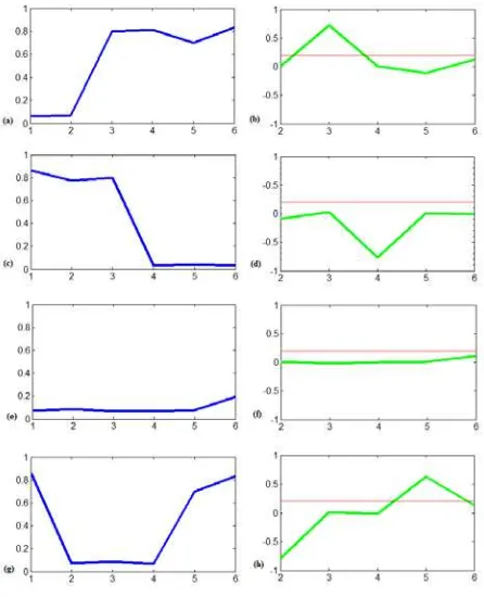
Each pixel (�,�) in the SITS is assigned six probability values, denoted as � (�,�,�), �= 1, … , 6. In order to show how and whether the probability value is increasing or decreasing, the first derivative (FD) of each pixel is calculated. The first derivative of a time series probability set is the slope of each time point, and can be described as
�� (�,�) =�(�,�,�)− �(�,�,� −1), �= 2, … ,6. (3)
The left column of Figure 4 reports the typical evolution in time of BPM values for a newly built building, a demolished building, unchanged ground, and a rebuilt building. The corresponding FDs are shown in the right column.
Figure 4. Evolution in time for the probability of a pixel to belong to a building: (a) newly built building; (b) FD of (a); (c)
demolished building; (d) FD of (b); (e) unchanged ground; (f) FD of (e); (g) rebuilt building; (h) FD of (g).
3.2 Object based YBC map generation
As illustrated in Tian et al. (2013), a main drawback of the DSM extracted from stereo imagery is the occurrence of imprecise height values in building boundary region and some texture-less surfaces. If a satisfactory segmentation can be performed, object-based methods work better than pixel-based ones for building change detection at high/ very-high resolution. We therefore segment the pansharpened image of the last date using the mean-shift approach (Comaniciu and Meer, 2002; Tian et al., 2013). The improvement of the BPM can be observed in Figure 5. We refer to the object-based regularized BPM as OBPM.
Figure 5. Comparison between BPM (a) and OBPM (b).
Theoretically the mean BPM value of each segment can be used to characterise the building probability at object level. However, influenced by the DSM quality, the accuracy of BPM in building boundary regions is lower than in other parts of the image. Thus, a pixel-object consistence check is proposed in this paper.
As shown in Figure 6 the 1st derivative based change check has been processed at both pixel and object level. A consistence check is designed by comparing the YBC maps generated from time series BPM and time series OBPM. The pixels which are not consistent between the two representations are marked as outliers and removed. Afterwards, the mean building probability of each object is recalculated by using the remaining pixels in the BPMs. We refer the refined OBPM as OBPMR.
Time series BPMs
YBC map - pixel based
Objects map
Time series OBPMs
YBC map - region based Consistence
check
Time series
OBPMR YBC map
Figure 6. Workflow of the object-based change class map generation.
4. RESULT AND EVALUATION
The performance of the proposed approach has been evaluated by comparing the results to the YBC reference map shown in section 2.3. Automatic building change detection aims at giving correct information about the location of the changed buildings and the year when the change happened. Therefore, in this part, two steps of evaluation are used. Firstly, the detected change mask is evaluated by comparing to the reference change mask
and pre-/ post-events data comparison results. In the second step, the obtained YBC map is compared to the reference YBC map described in section 2.3.
4.1 Time series BPMs
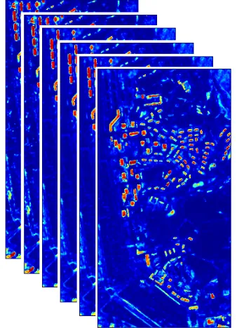
BPMs for all SITS are generated based on the method explained in section 2. The values in each BPMs ranging from 0 to 1 represent the probability for each pixel of belonging to buildings. As shown in Figure 7, the generated BPMs describe clearly the distributions of the buildings, and most of the buildings are well separated from others.
Figure 7. Generated time series BPMs
4.2 Change mask evaluation
As described in section 3.1, the determination of a threshold � is required to obtain an YBC map from the FD feature of the BPM. In this experimental section, a low threshold �= 0.2 is given to preserve more changes in the pixel-object YBC check procedure. The generated outlier mask is shown in Figure 8 (b).
(a) (b)
Figure 8. Generated change mask evaluation result (a) (Green: true detected; red: false positive; blue: false negative; black:
As illustrated, most of the outlier pixels, represented in white, are located in the building boundary region. Some of these pixels might be parts of the building segments. Figure 8(a) shows the result by giving a threshold value �= 0.3 to OBPMR. The detected change mask is overlaid to the truncated YBC reference map. That implies that only change and non-change areas are of interest in this evaluation procedure. In Figure 8 (a) the correctly detected changes are marked in green, red represent false positives, and blue represent false negatives.
However, the accuracy of the change mask depends strongly on the given threshold values. Therefore, the change detection results obtained using time series BPMs, OBPMs, and OBPMRs are compared by plotting the Kappa Accuracy (KA) obtained with 100 threshold values ranging from 0.01 to 1 �� ( ��= 0.01, 0.02, 0.03, … , 1).
Figure 9 shows the KA curves. As expected, the OBPMR (black line) is more robust and less dependent on the given threshold values. The obtained KAs are generally higher than 0.6 when the threshold values are ranging from 0.1 to 0.6. The results for OBPM (green line) are generally not as good as for OBPMR, but they outperform the ones derived from the original BPMs (red line). An accuracy decrease can be observed for OBPM (green line), as OBPM takes the average value for each object, some changed objects may be shown as false negative when a higher T is given. However, the accuracy is improved after the consistence check (black line).
Figure 9. KA comparisons for change masks.
In addition, the change map for a single data pair (pre- and post-event) is generated and evaluated. We generate a difference map
���� (����=���6− ���1), using the BPMs from the earliest and the latest dates (BPM1 and BPM6, respectively). The pixel values in BPMs range from 0 to 1, thus the accuracy of
���� can be plotted on the same chart by using the same �� set. The blue line shows the derived KA curve. The BPM yields a satisfactory performance, as both special and temporal information are exploited in its generation. Nevertheless, the highest accuracies are obtained for values of T between 0.1 and 0.7, and in this range OBPMR outperforms BPM.
The advantages of the time series are well proved for some special buildings. The yellow box in Figure 8 locates some correctly detected changed buildings. However, three of these are not properly highlighted in the BPM6, as shown in Figure 10 (a). Thus, a direct subtraction of the two BPMs as reported in Figure 10 (b) is not able to correctly detect these changed buildings.
Figure 10. BPM6 (a) and DIFF (b) of the sub-region marked in Figure 8 (a).
4.3 YBC map evaluation
With the same threshold value (�= 0.3), a YBC map is generated and displayed in Figure 11. It shows that most of the blue buildings match well with the YBC reference map (Figure 3). The evaluation has been performed as in the change mask
evaluation procedure. A series of
�� ( ��= 0.01, 0.02, 0.03, … , 1) are used to plot the KA curve. In Figure 12, the black line describes the accuracy of OBPMR generated with ��. As a comparison, YBC maps are also derived from BPMs and OBPMs. The KA values are plotted with red and green lines in Figure 12. Since the DIFF map is not able to retrieve as detailed YBC information as the series maps, this is not included in this comparison procedure.
Figure 11. Detected change class map (Blue: built before 2009; Yellow: built before May 2010; Orange: built before January
2011; Darkred: built before May. 2011).
Figure 12. KA comparisons for YBC maps.
Some errors are detected if the building probability values in one date are wrong. In Figure 11, some buildings changed in year 2009 are wrongly labelled. The building probability series values of the building marked with a black circle are shown in Figure 13 (a). As it can be seen, this building is actually built before 2009. However, in the fifth dataset (Jan. 2011), this building has a very low value in the BPM map. Thus, it was detect as newly built building in the year 2011. The FD in the sixth date, however, is higher than the FD in the second date. Removing this kind of false alarm is not an easy task: such rapid variations may be justified in some cases, as in some rapidly growing developing cities some buildings could be rebuilt twice within ten years.
Figure 13. Building with incorrect change class (Blue: building probably series values; Green:FD; Red: Threshold line).
5. DISCUSSION AND CONCLUSIONS
Detecting single building changes from satellite images is becoming possible with the growing availability of VHR satellite imagery, such as IKONOS and WorldView-2. This study demonstrated that SITS stereo data can be used to generate a detailed and robust building change detection task.
As buildings are off-terrain objects, height has been proved to be a direct and reliable feature for extracting building changes. Compared to LiDAR data, satellite stereo data are advanced in two aspects: the large swath and the availability of intensity (panchromatic) and colour (multispectral) information. Unfortunately, the DSMs generated from stereo data are not yet as accurate as the ones derived from LiDAR datasets, and some buildings might have incorrect information if the matching fails to capture the height of the roof pixels. Some change detection methods based on stereo images may reduce some errors for small-size buildings. Approaches in Tian et al. (2015) are helpful to remove some false positives, but it is very challenging to avoid false negatives. A new building cannot be included in the final change mask, if it is not displayed as an off-terrain object in the post-event DSM.
This paper has presented a robust approach for detecting and characterizing building changes in SITS. The adopted building probability map generation approach and further developed time-series data analysis method are robust and can be easily applied to any multi-sensor and multi-seasonal SITS dataset.
Furthermore, only a few threshold values are required, and the final results are not very sensitive to them. As further work, the time series analysis algorithm can be improved by including temporal resolution and sizes of the objects as weights in the frame of an adaptive process.
REFERENCES
Benediktsson, J., A., Pesaresi, M. and Amason, K., 2003. Classification and feature extraction for remote sensing images from urban areas based on morphological transformations. IEEE
Transactions on Geoscience and Remote Sensing 41 (9), pp.
1940-1949.
Bontemps, S., Bogaert, P., Titeux, N., and Defourny, P., 2008. An object-based change detection method accounting for temporal dependences in time series with medium to coarse spatial resolution. Remote Sensing of Environment 112(6), pp. 3181-3191.
Breiman, L., 2001. Random forests. Machine learning 45 (1), pp. 5-32.
Chen, B., Xu, G., Coops, N. C., Ciais, P., Innes, J. L., Wang, G., ... and Liu, Y., 2014. Changes in vegetation photosynthetic activity trends across the Asia–Pacific region over the last three decades. Remote Sensing of Environment, 144, pp. 28-41.
Comaniciu, D., Meer, P., 2002. Mean-shift: a robust approach toward feature space analysis. IEEE Transactions on Pattern
Analysis and Machine Intelligence 24 (5), pp. 603–619.
de Jong, R., de Bruin, S., de Wit, A., Schaepman, M. E., & Dent, D. L., 2011. Analysis of monotonic greening and browning trends from global NDVI time-series. Remote Sensing
of Environment, 115(2), pp. 692-702.
Fensholt, R., and Proud, S. R., 2012. Evaluation of earth observation based global long term vegetation trends— Comparing GIMMS and MODIS global NDVI time series.
Remote sensing of Environment, 119, pp. 131-147.
Hirschmüller, H., 2008. Stereo processing by semiglobal matching and mutual information. IEEE Transactions on
Pattern Analysis and Machine Intelligence 30 (2), pp. 328-341.
Huang, X., Zhang, L. and Gong, W., 2011. Information fusion of aerial images and LIDAR data in urban areas: vector-stacking, re-classification and post-processing approaches.
International Journal of Remote Sensing 32 (1), pp. 69-84.
Jolliffe, I., 2005. Principal component analysis. Encyclopedia of
Statistics in Behavioral Science 3 (1), pp. 1580-1584.
Lowe, D. G., 2004. Distinctive image features from scale-invariant keypoints. International Journal of Computer Vision 60 (2), pp. 91-110.
Qin, R. and Fang, W., 2014. A hierarchical building detection method for very high resolution remotely sensed images combined with DSM using graph cut optimization.
Photogrammetric Engineering and Remote Sensing 80 (8),
37-48.doi: 10.14358/PERS.80.9.000
Qin, R., Huang, X., Gruen A. and Schmitt, G., 2015. Object-based 3-D building change detection on multitemporal stereo images. IEEE Journal of Selected Topics in Applied Earth
Observations and Remote Sensing 5 (8), 2125-2137.10.1109/JSTARS.2015.2424275
very-high-resolution space-borne stereo images. International
Journal of Remote Sensing, pp. 1-22.
Tian, J., Reinartz, P., d’Angelo,P., and Ehlers, M., 2013. Region-based automatic building and forest change detection on Cartosat-1 stereo imagery, ISPRS Journal of Photogrammetry
and Remote Sensing 79, pp. 226-239.
Tian, J., Cui, S., and Reinartz, P., 2014. Building change detection based on satellite stereo imagery and digital surface models. IEEE Transactions on Geoscience and Remote Sensing 52(1), pp. 406-417.
Tian, J., Dezert, J., and Reinartz, P., 2015. Refined building change detection in satellite stereo imagery based on belief functions and reliabilities. 2015 IEEE International Conference
on Multisensor Fusion and Integration for Intelligent Systems
(MFI), pp. 160-165.
Verbesselt, J., Hyndman, R., Newnham, G., & Culvenor, D., 2010. Detecting trend and seasonal changes in satellite image time series. Remote sensing of Environment 114(1), pp. 106-115.
Yang, X., and Lo, C. P., 2002. Using a time series of satellite imagery to detect land use and land cover changes in the Atlanta, Georgia metropolitan area, International Journal of