CHAIN-WISE GENERALIZATION OF ROAD NETWORKS USING MODEL SELECTION
Dimitri Bulatova, Susanne Wenzelb, Gisela H¨aufela, Jochen Meidowa
aFraunhofer IOSB, Ettlingen, Germany, [email protected] b
Institute of Geodesy and Geoinformation, Photogrammetry Group, University of Bonn, Germany, [email protected]
Commission II, WG II/IIII
KEY WORDS:Road Extraction, Generalization, Polyline Simplification, Model Selection, Traffic Roundabout
ABSTRACT:
Streets are essential entities of urban terrain and their automatized extraction from airborne sensor data is cumbersome because of a complex interplay of geometric, topological and semantic aspects. Given a binary image, representing the road class, centerlines of road segments are extracted by means of skeletonization. The focus of this paper lies in a well-reasoned representation of these segments by means of geometric primitives, such as straight line segments as well as circle and ellipse arcs. We propose the fusion of raw segments based on similarity criteria; the output of this process are the so-called chains which better match to the intuitive perception of what a street is. Further, we propose a two-step approach for chain-wise generalization. First, the chain is pre-segmented using circlePeuckerand finally, model selection is used to decide whether two neighboring segments should be fused to a new geometric entity. Thereby, we consider both variance-covariance analysis of residuals and model complexity. The results on a complex data-set with many traffic roundabouts indicate the benefits of the proposed procedure.
1. INTRODUCTION AND PREVIOUS WORK
Roads are very important entities of any geographic database. Since they are man-made objects, road networks exhibit, often and particularly in urban terrain, regular structures, e. g., straight lines, circles, clothoids, ellipses, as well as orthogonality and symmetry. However, automatic detection of these regularities from airborne captured image or laser data is difficult. Occlusions and shadows are probably the most intuitive challenges when one thinks about road extraction. In fact, roads mostly are occluded by tree crowns, balconies of buildings, or (groups of densely) parking vehicles and their shadows. This is where semantics be-comes relevant: Which obstacles can be ignored and which can-not? A separation line between two highway directions may look similar to a queue of trucks, hence, differentiation between both groups of objects should ideally be made. The third aspect, valid in case of aerial images, is that roads have often very homoge-neous textures as well as moving objects; hence noise and outliers often make acquisition of 3D information difficult. However, el-evation data, extractable, for example by means of depth maps (Rothermel et al., 2012), has turned out to be essential for recon-struction of roads in urban terrain (Hinz and Baumgartner, 2003; Wegner et al., 2015).
All these challenges let the automatically extracted road networks – which are mostly stored in geographic bases in form of vec-tor data for street centerlines – appear extremely wriggled and should be corrected or generalized within a post-processing step. There are several contributions related to generalization of road networks but for most of them, Chaudhry and Mackaness (2006) for example, data noise is not a significant problem. Our work is more similar to (Bulatov et al., 2016b; Mena, 2006), where segments are extracted from the actual sensor data and finally generalized either by the well-known algorithm of Douglas and Peucker (1973) or by higher order, e. g., B´ezier curves. Both modules (Douglas-Peucker and B´ezier curves) were modified in the way that the polygonal chains do not cross obstacles, such
as buildings and trees. There are two major drawbacks of this approach: Neither variance-covariance error analysis was carried out nor any kind of hypothesis testing which of two models – a straight line or a smooth B´ezier curve – is actually relevant for the current segment. Besides, the approach was applied to very short segments that are defined between two branch points result-ing from a skeletonization algorithm. The effect of generalization was thus barely visible, in particular, because segment endpoints are fixed.
It is well-known, however, that for road nets, not only geomet-ric but also topological correctness, that is, connectivity between roads, becomes extremely relevant. Several authors (T¨uretken et al., 2013; Wegner et al., 2015) exploited this fact for road extrac-tion and in this work, we exploit topology for post-processing. We establish neighborhoods between segments and generalize chain-wise. The advantages are on the one handsemantic– since the chains satisfy better the intuitive notion what a street is – and on the other handgeometric, since more points are considered for the upcoming generalization, increasing thus the redundancy. The process of generalization itself consists of fitting geometric primitives, namely, straight line segments, circle and ellipse arcs into chains of points. We first create an over-segmentation of cir-cular segments using a modified version of Douglas and Peucker (1973) and finally merge neighboring segments using iterative model selection.
We ought to mention that the problem of fitting geometric primi-tives in pixel chains and 2D meshes has been extensively treated in the past. For example, G¨unther and Wong (1990) propose the so-called Arc Tree, which represents arbitrary shapes in a hierar-chical data structure with small curved segments at the leaves of a balanced binary tree. Moore et al. (2003) propose a method for polygon simplification using circles. They aim at closed poly-gons given by a set of 2D points. Finding ellipses in images has attracted many researchers (Porrill, 1990; Patraucean et al., 2012). But these works start from pixel-chains, which is not the case in our application. We are interested in the more general
This contribution has been peer-reviewed. The double-blind peer-review was conducted on the basis of the full paper.
problem of describing polygonal chains by sequences of straight line, circle, and ellipse segments, a problem which was similarly addressed in Albano (1974), however, neither enforcing ellipses, nor looking for a best estimate for ellipses.
Most related to our approach is the work by Rosin and West (1995) where segmentation of point sequences into straight lines and ellipses is performed within a multistage process. Model se-lection is done implicitly by evaluating a significance measure to each proposed segment, which is based on its geometry, purely. However, their criteria are non-statistical, thus, cannot easily be adapted to varying noise situations. Ji and Haralick (1999) crit-icize this and modified their idea by a hypothesis testing frame-work. Again, these approaches are applied to images and pixel chains, respectively.
The main contribution of this work is to combine thesemantical approach of fusing road segments and assuming that they – as a typical man-made object – can be approximated by some geo-metric primitives with thestatisticalapproach of model selection which allows to decide whether neighboring segments can be rep-resented by a single primitive. The approach of model selection is based on information theory since not only coordinates’ resid-uals but also model complexity is taken into consideration. Note that after the generalization, the data is not necessarily consistent anymore; for example, lines and circles are not guaranteed to in-tersect. However, the adjacency information is not lost and can be used to create junctions of appropriate size so that the geometric inconsistencies are not visible. This is exactly the way the road networks are managed in most urban terrain simulation systems and many other applications.
For reasons of completeness, we provide in Sec. 2 a brief sum-mary of methods we applied in order to fit geometric primitives, such as straight lines, circles, and ellipses. By ellipses, we strive to approximate clothoides, which are more often employed to provide a smooth transition of curvature for curvy road courses; however, clothoids turn out to be less handy for the chain form-ing module. The process of chain formform-ing, applied once a raw road network had been extracted from the classification result, is explained in Sec. 3. In Sec. 4, we present our algorithm on chain-wise generalization. Our results in Sec. 5 verify that road networks generalized chain-wise with multiple primitives are vi-sually more appealing than the results of segment-wise general-ization with multiple attributes. In Sec. 6, main conclusions and ideas for future work are provided.
2. BASICS
Given the set ofN observed points
X
= {xn}, n = 1. . . N, we aim at the best fitting straight line, circle or ellipse, which we represent as homogeneous elements. In each case, we look for the statistically best fitting parameter vector as well as its co-variance. We need this when merging neighboring lines based on their statistical properties. A detailed discussion of uncer-tain homogeneous points and lines can be found in F¨orstner and Wrobel (2016) and Meidow et al. (2009). We assume i.i.d. co-ordinates of each point, sharing the same isotropic covariance Σxnxn=σ 2
nI2.
Straight Line In (F¨orstner and Wrobel, 2016, Sec. 9.4.2), it is shown that the statistically best fitting line passes trough the cen-troid of given points and that its direction is given by the principal axis of their moment matrix. We obtain the estimated homoge-neous coordinates of linebland the covariance matrixΣblbl.
Ellipse We use the homogeneous representation of conics to express the parameters of the ellipse. Thereby, we represent con-ics with the symmetric3×3-matrix
C=
For estimating the parameters we use the implicit polynomial representation of the conicyTc = 0, with the vector of
un-knownsc = [c11, c12, c22, c13, c23, c33]Tand the
observa-tionsy = [x2,2xy, y2,2x,2y,1]T.To ensure the conic to
be an ellipse,|Chh|>0must be fulfilled. Thus, we impose the quadratic constraintc11c22−c
2
12 = 1, which is a valid choice,
as the conic representation is homogeneous and all parameters can be divided by any zero scale factor. This leads to a non-linear Gauss-Helmert model. Using initial parameters estimated by means of the direct method of Fitzgibbon et al. (1999), we follow Wenzel (2016, Sec. 2.1.3, p. 47ff) to obtain the estimated parametersbcof the conic and their covariance matrixΣbcbc.
Circle A circle is a special regular conic for which the matrix Chh ∝ I2in (1). Instead of using the over-parametrized conic representation, we represent circles by their implicit homoge-neous equationzTp = 0, where we collect the coordinates of a pointxin a vectorz = x2+y2, x, y, 1T
and the param-eters within vectorp= [A, B, C, D]T, from which we easily
obtain the circles parameters,x0, y0, r. Note that settingA = 0
allows us to represent circles with infinite radius, thus, straight lines. Given at least three observations, the resulting linear equa-tion system can be solved using a SVD-based method, which we refer on as direct method. Instead, we follow F¨orstner and Wro-bel (2016, Sec. 3.6.2.5) and derive the covariance matrix of the circles’ parameters[x0, y0, r]directly from observed points.
Fi-nally, using variance propagation, we yield estimated parameters
b
pand the according covariance matrixΣbpbp.
3. ROAD-NET EXTRACTION AND CHAIN FORMING
Usually, classification results are represented by binary maps. The first step of our pipeline thus consists of vectorizing these maps. We obtain a set of polygonal chains, to which we will re-fer as polylines. The result may appear noisy and thus, we must filter out those polylines which do not correspond to our under-standing of what a (part-of-a-)road is. These steps are explained in Sec. 3.1. Our next task is fusion of the remaining polylines into chains, which is done for two main reasons. Firstly, since the polylines connect just neighboring junctions, the chains conform better with our perception of street than the raw polyline. Think about the Oxford Street in London. Its name remains the same throughout its course, even though multiple side roads decom-pose it into several polylines. Secondly, chains are more suitable for generalization, since the whole geometry of the entity may be captured. More details are explained in Sec. 3.2. The contents of this section are visualized on a running example in Fig. 1.
3.1 Vectorization and Extraction of Road Polylines
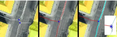
Figure 1: Main steps of chain forming algorithm. Left: vectoriza-tion by means of medial axis; forbidden areas are indicated by the golden color. Middle: The implausible segments are filtered out. We also recommend fusing junctions (denoted by blue crosses) in order to increase the number of neighbors for chain forming (right image). Two segments are fused into a chain (cyan), because their partial dominant direction were similar. The red segment is a side road in this case. Chains and side roads are the main input for the chain-wise generalization, see Sec. 4.
is a set of open polygonal chains, which we call polylines. An endpoint of a polyline is always either a pixel on∂B(usually, any concavity), or a branch point, for which at least three points, belonging to∂B, have the same distance. In the first case, we re-fer to the polyline endpoint as to adead endwhile in the second case, we denote it as ajunction. Beside these two cases, a partic-ular situation is observed if the polyline is closed, or, equally, if it is homeomorphic to the circular line. In this situation, both dead ends coincide with one of the vertices of the polyline.
To recognize whether a polyline endpoint is a dead end or a junc-tion, the range-search procedure is applied. All endpoints are clustered by means of the generalized DBSCAN algorithm (Sander et al., 1998), which is the state-of-the-art tool for downsampling point clouds. A junction is a cluster with at least three vertices. The structure of junctions contains their 2D coordinates and the corresponding incident polylines. Since every concavity of B
causes one polyline, discarding those road segments which ex-hibit a suspicious geometric appearance (too short, too broad, etc.) and at the same time do not contribute to the topologi-cal functionality of the road net has been proposed in the liter-ature (Mena, 2006; Bulatov et al., 2016b). Thus, the iterative filtering procedure is based on polylineattributes, such aswidth, length, type, etc., which are calculated according to Bulatov et al. (2016a). More concretely, we delete within one iteration all poly-lines of which at least one endpoint is not a junction and whose length or width take on a suspicious value (e. g., the length below 2 m or width out of range [2 m; 50 m]). After every iteration, the attributes are updated. In order to remove redundant loops, for example, around isolated trees, an additional module was im-plemented, however, not employed since we wish to demonstrate the tools implemented in the next section to fit circle arcs.
3.2 Chain Forming
The previously discussed polylines serve, for the most part, as connection links between the junctions and do not correspond to the generally understood term of street. We wish to perform fusion of polylines into chains in order to generalize them chain-wise in the next step. The essential precondition of chain form-ing is establishform-ing – geometric and topological – similarities be-tween the polylines, which is done using the attributes mentioned in Sec. 3.1. That is, to find candidates for fusion, we have to search for similar attributes between pairs of polylines. The nec-essary condition for similarity is that two polylines are topolog-ically neighboring; in other words, they must share a common
junction. This additionally simplifies the implementation since all the remaining steps of the algorithm run over junctions. Given two polylines gathered in a junction, the (dis)similarity of their geometric attributes is denoted ascost. The smaller the cost, the larger the likelihood of two polylines to be merged. After all
n(n−1)/2costs are collected, wherenis the number of polylines converging to a junction, pairs of candidates with minimum cost are collected for the upcoming fusion process. This may be done either by a greedy algorithm or using the Hungarian Method. We opted for the former one, our choice because of its simplicity and because only a few values ofnexceed 4. The order of vertices of the merged polylines should be topologically correct. This means on the one hand, reordering the polyline segments to be fused and, on the other hand, flipping the order of points within one polyline, if necessary.
In the rest of this section, we outline different methods for com-paring geometric attributes keeping in mind that we want to iden-tify both straight and circular chains. First of all, we established a width gap: The necessary condition for two road segments to be neighbors is that the width of the narrower one, denoted bywmin,
and that of the broader one,wmax, are similar, that is
(1−ε)wmax< wmin, whereε≈0.5. (2)
This assumption is reasonable because a street usually has a con-stant width throughout its course. Note that even though this threshold may seem large, it is only a necessary condition. To make this condition also sufficient, we investigated two promis-ing methods: First, thepartial dominant directionsof two neigh-boring polylines and second, the direct circle-fit method from Sec. 2 within a RANSAC framework (circle-fit + RANSAC).
In order to estimate the partial dominant directions, we build for each polyline a weighted histogram of directions modulo 180◦, where the weights are proportional to the segments’ lengths. A hill-and-dale analysis of the smoothed histograms yields, in es-sential, the partial dominant directions. Our cost function is thus given by the truncated absolute difference of the partial dominant directions corresponding to the relevant junction (Fig. 1, right). The more the dominant directions differ, the higher the cost.
For the second approach, the direct circle-fit method mentioned in Sec. 2 is the core function for the RANSAC algorithm over the union of vertices of both polylines. Here the dissimilarity is given by the percentage of outliers. The advantage of this method is that we can detect, consciously, circular structures around a junction. The problem, however, is extension of chains over pairs of polylines without storing the parameters of the fitted circles. Note that numerous further cost functions can be devised. Be-sides those mentioned in Bulatov et al. (2016a), we implemented the circle-fit function from the minimum set (the junction and two loose ends) of both polylines and measured once again the outlier percentage to build the cost function. Clearly, this was by far less accurate than the solution based on RANSAC. Alternatively, one could compare the curvatures of the adjacent polylines. However, the positions of vertices are often very noisy and, since building the second derivatives is hardly known to be a numerically stable process, we rejected this idea. Summarizing, partial dominant di-rections and circle-fit + RANSAC, both preceded by the width gap filter, are the best trade-offs between characterization of the local course of the polyline near the junction and the point of view of the numerical stability, for which possibly all vertices should be considered.
This contribution has been peer-reviewed. The double-blind peer-review was conducted on the basis of the full paper.
4. GENERALIZATION
Given the chains from road-net extraction, we wish to represent them by sequences of straight line, circular, and ellipse segments. The proposed method consists of two steps, described in subsec-tions 4.1 and 4.2. Given the chains, we first iteratively segment them into circular segments, which yields an over-segmentation. Second, merging neighboring segments is performed based on model selection. In this step, straight lines, circular arcs and ellipses are estimated optimally in a least squares sense. This way, we are more flexible representing curved courses than us-ing straight lines, solely. It might be confusus-ing that polylines just connected to chains are segmented into smaller parts again, which are then fused once more. Note that the chain-forming procedure is based on topology and the streets attributes, while pre-segmentation here is just based on the polylines geometry. Over-segmentation is a natural side-effect of the algorithm and is desired in order to generate proposals for later merging to larger and potentialy more complex geometric objects, which are con-sistent to the given raw data on one hand but generalizations in terms of our intuition of streets on the other hand.
4.1 Segmenting Point Sequences into Circle Segments
The concept of chain segmentation into circle segments is based on thecirclePeuckeralgorithm (Wenzel and F¨orstner, 2013), which is an adaption of the well known Douglas-Peucker algo-rithm (Douglas and Peucker, 1973). The original algoalgo-rithm is designed to simplify polylines by recursively splitting a sequence of polyline edges into larger edges until the distance of an elimi-nated point to the corresponding edge is below a thresholdt.
Instead of straight lines,circlePeuckeruses circle segments (Wenzel and F¨orstner, 2013). Given a sequence of points, it is recursively partitioned into segments which approximate the ac-cording points by a circular arc up to a pre-specified tolerancet. If applicable, a segment is split at that point
x
n, where the dis-tance to the circular arc is maximum. In order to enforce continu-ity, they fix the start and endpoint of the segments and determine the best fitting arc. As thresholdtwe use in our application half of the width of the smallest street part involved in the relevant group; the width gap mentioned in Eq. (2) widely guarantees uni-formity of width values. As result we obtain a list of indices which represent the endpoints of sought segments. This yields the required partitioning of the original point sequence.4.2 Merging Line Primitives Based on Model Selection
Given the preliminary, over-segmented partition of the chain, we aim at a simplification by merging neighboring segments which share the same geometric model instance. Deciding whether two neighboring segments belong to the same model instance may be based on a statistical hypothesis test. As these tests aim at re-jecting the null hypothesis, they can be used as sieve for keeping false hypotheses. Merging segments merely based on hypothesis testing, however, fails due to the risk of accepting large changes in geometry, in case the parameters of the proposed model are uncertain. On the other hand, deciding which model fits the data best, i. e., whether it should be approximated by a straight line, circle or an ellipse, is a typical model selection problem.
The domain of models we use is{straight line, circle, ellipse}, which differ in the number of parameters. Here the term accu-racy is related to the residuals, v, caused by deviations of the points to the selected model. Let us consider a number ofN
normally, i. d. observationslwith covarianceΣll. We are look-ing for anU-dimensional parameter vectorθb, whereby observa-tions and parameters are related by the Gauss-Markov functional modell+vb=f(θb). Using the usual definitionΩ =bvT
Σ−1
ll vb, Schwarz (1978) derived the Bayesian Information Criterion
BIC= Ω +UlnN , (3)
as a criterion for model selection. The lower the complexity of the model, given by the number of parametersU, the lower BIC. A large numberNof observations increases the relative precision of the parameters and thus the reliability of the model. It can be shown that the BIC is closely related to thedescription length from information theory. Thus, we use these terms synonymously and wish to minimize Eq. (3) to select the best model.
From the pre-segmentation, we only take the information which points belong to the same segment and ignore the parameters of the fitted circle segments. The final representation is achieved by fitting straight line, circle and ellipse segments through chains and side roads, respectively, using all points belonging to them. Again, given a set ofNobservations
X
={xn}, n= 1. . . N, where we assume i. i. d. coordinates of each point, sharing the same isotropic covarianceΣxnxn=σ
0 in order to scale the variance of observations.
For each model, we look for the statistically best fitting parameter vector as well as its covariance by estimating the weighted sum of squared residualsΩ =Pnbv2
n/σ
2
nas measure of precision and the estimated variance factorbσ2
0 = Ω/(N−U).
Let us assume a segmentation of points
X
={X
m}intoM seg-ments. We call the current parameter vector of them-th segment θm. Thus,θmacts as placeholder forlm,pmorcmand includesthe numberUmof parameters (2,3, and5respectively) needed to define the current model, which is our measure of complexity. Initially, we select the best model for each segment by minimiz-ing its description length in terms of the BIC
b ments by evaluating the gain of description length when fitting a new model to the joined set of points. Assume that we al-ready found modelsθbmandθbm+1using the points
X
mof seg-mentmandX
m+1of segmentm+ 1, respectively. We proposethe points of both segments to belong to a joined segment, thus,
X
m,m+1 =X
m∪X
m+1. Again, we select the best model, forthis potentially merged segment, by minimizing the BIC
b
θm,m+1= argmin
θ
m,m+1
BIC(
X
m,m+1,θm,m+1) . (5)The gain of description length is given by the difference between the joint description length using the model θbm,m+1 obtained
with the merged segments
X
m,m+1and the sum of descriptionsIf∆BICm,m+1>0the description length of the merged segment
is shorter than the description length of two separate segments; thus, they should be merged to reduce the overall complexity.
To evaluate the whole set of segments, we proceed in a greedy manner. After initializing all segments by their best models in terms of description length, we propose all neighboring segments to be merged and select the according best model. From all neigh-bored pairs which have a positive gain of description length, we select the one with the largest gain. We update the segmentation, such that one break point is removed. We iterate this process until there are no more merging proposals with positive gain of description length.
Finally, we inspect the estimated variance factorsσb2
0 of the
fi-nally merged segments. If they deviate more than10%fromσ2 0,
the initial variance of observations was too optimistic or too pes-simistic, respectively. Thus, we considered restarting the process, usingσ′
0 =σb0·σ0. Hence, the final segmentation adapts to the
given data and to the specific characteristic of each road segment. We refer to this variant of generalization asadaptiveversion.
Note that the resulting partitioning may deviate from the original junctions, as in the adjustment procedures the geometric elements are not restricted to any particular points. However, the covari-ance matrices for junction points – introduced at the beginning of Sec. 2 – could be re-weighted in order to prevent the according points changing their positions, in terms of their residuals. This is part of our future work.
5. RESULTS
To evaluate the accomplished work, we considered the dataset from the inner city of Munich, Germany. Given several aerial panchromatic images enriched by near infrared channel, a dig-ital surface model and an orthophoto were calculated using the method of Rothermel et al. (2012). The resolution of the or-thophoto was around 0.2 m. To perform classification, we first computed the digital terrain model by a standard procedure, which comprises extraction of several ground points followed by a spline interpolation and is described in (Bulatov et al., 2014). Then we excluded right away the set offorbidden pixelswith implausible values of relative elevation and NDVI. Finally, we extracted some regions for training and evaluation procedure. Besides, we used stripes computed from pairs of nearly parallel lines in orthophoto to suppress the noise stemming from vehicles, traffic signals, etc.: If at least a certain percentage of pixels belongs to the road class, all other non-forbidden pixels are also assigned to the street class. There are still many mis-classifications in this difficult dataset. However, especially by choosing regions for training data extrac-tion, we made sure that road pixels are extracted as correct as possible in the regions around the traffic roundabouts since this is where we want to demonstrate the performance of our algorithm.
In Fig. 2, we show two fragments of the dataset with classifi-cation result, the extracted polylines (chains are omitted), and the content of the shapefile obtained from a publicly available source Geofabrik (2017). These images show on the one hand the achievable accuracy of our street extraction module in com-parison with the ground truth and on the other hand, the problem-atic of the wriggled road courses, which we will improve next. Thus, we will show in Sec. 5.1 the process of chain forming and in Sec. 5.2, we assess the results of generalization.
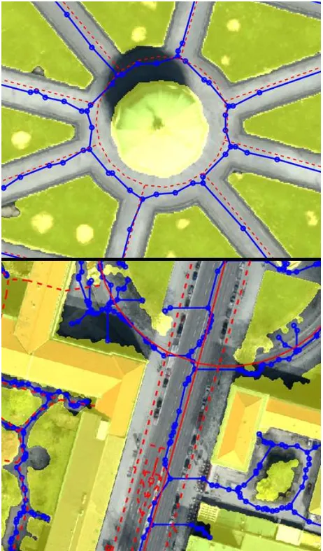
Figure 2: Detailed view of the classification results, where non-road class is emphasized by golden color, the input polylines, in blue, and the “ground truth” represented by the content of the OpenStreetMap shapefile, in red. Here, main and auxiliary roads are depicted by solid and dashed lines, respectively.
5.1 Chain Forming
We show in Figs. 3-4 the performance of both strategies for dis-similarity searching, namely by means of RANSAC outliers of the circle-fit function and deviations in partial dominant direc-tions. The polylines not belonging to any chain (equivalently, to chain of cardinality one) will be denoted from here on asside roads. They are omitted in Fig. 3 and marked by thin cyan lines in Fig. 4. We see that the strategy based on fitting circles is bet-ter suitable for searching circular regions than comparing partial dominant directions. Thus, the circle in Fig. 4, right, has been correctly determined. However, in general, the function based on partial dominant direction tends to identify more natural street courses, which is best visible in Fig. 3, right, otherwise chains formed by straight lines become more easily interrupted. For re-gions not reasonable for generalization, such as foot paths, high-lighted in Fig. 4, right, both methods exhibit rather short and senseless chains. Since only direct neighbors are considered for chain forming, situations where small segments appear between two junctions are undesirable, as well and should be avoided by means of DBSCAN. It remains to say that circle-fit + RANSAC is
This contribution has been peer-reviewed. The double-blind peer-review was conducted on the basis of the full paper.
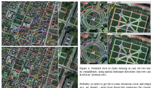
Figure 3: Results of chain forming with neighborhood searching function based on partial dominant directions (top) and on circle-fit + RANSAC (bottom), visualized for the complete dataset (left) and a for long street (right). The chains are given random, arbi-trary colors. Side roads were omitted.
a slightly more time consuming strategy than the histogram anal-ysis needed for estimation of partial dominant directions (around 20% of time) and the main problem of the latter method is made up by noisy assignments of directions to the individual segments.
5.2 Generalization
We processed once the chains and once the side roads with the adaptive and non-adaptive version of generalization. In what fol-lows, the differences between the results as well as their depen-dencies on the underlying function for neighborhood search will be analyzed. We observe in Fig. 5 that by using the adaptive version of generalization, straight line segments often tend to be approximated by groups of circle arcs while circle arcs are likely to be approximated by ellipses. This is due to the fact that model selection tries to solve the trade-off between precision and model complexity. Down scaling the assumed accuracy of observations leads to smaller residuals and more complex geometries. We can also see that the gap between the endpoints of a neighboring el-lipse and a line is often smaller than in case of circles. Com-ing to the comparison of underlyCom-ing function for neighborhood search, we see that after the approach based on partial dominant directions, several circle arcs belonging to the traffic roundabout in Fig. 5, top, are lost, however not many, and that the whole circle could not be recognized in Fig. 5, third row. Application of circle-fit + RANSAC allows extracting this circle completely (within the non-adaptive approach). As a disadvantage, we can see in Fig. 5, second row, some hallucinated circle and ellipse arcs. Additionally as described in previous section, long straight streets are sometimes interrupted and the slopes of the single re-gression lines are not identical.
Figure 4: Detailed view of chain forming in case for two traf-fic roundabouts, using partial dominant directions (top row) and RANSAC (bottom row).
Probably, in order to get rid of some erroneous circle and ellipse arcs, we should – apart from drastically improving the classifi-cation result – consider clothoids instead of ellipses. They are known to be an essential part of design of road geometries, they have less degrees of freedom than ellipses and they would per-fectly fit in our model estimation and selection procedure from Sec. 2 and 4.
To demonstrate the advantages of fusion with respect to the pre-vious approaches, Fig. 6 shows the results of application once of the generalization module based on multiple primitives (circle-fit-based, non-adaptive) butwithout fusion, visualized by dashed red straight lines and yellow circle arcs and once the result of polyline-wise Douglas-Peucker algorithm modified by Bulatov et al. (2016b), shown by blue line segments. As expected, the latter approach extremely compresses the number of vertices and the junction positions remain fixed, yielding sometimes slant road courses. This usually does not happen with red lines, since these result, basically, from a regression procedure. However, junction positions are not fixed anymore. Also, the former method tends to recognize, where possible, circle arcs, which sometimes make the road course more realistic, but sometimes stem clearly from the noise. Besides, because there are usually not enough observa-tions in a single polyline, these circle arcs were more difficult to recognize than with chain-wise method visualized in Fig. 5 and the traffic roundabouts are not recognized that clearly. Summa-rizing, both alternatives do a fair job when it comes to general-ize straight lines, however, in order to identify circular segments, polyline fusion seems to be indispensable.
6. CONCLUSIONS AND OUTLOOK
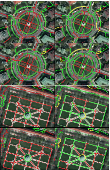
Figure 5: Detailed views of generalization results from two traffic roundabouts. The output of non-adapted and adapted generaliza-tion is shown, respectively, in the left and in the right images. The output of partial dominant directions and circle-fit + RANSAC is shown, respectively, in the top and in the bottom images. All el-ements stemming from a chain are highlighted with solid lines while the side roads are represented by dashed lines. We show the resulting circle and the ellipses arcs as well as the straight line segments by green, yellow, and red color, respectively.
cases, roads corresponding to both polylines are required to have similar width and to share a junction. Using a greedy approach based on model selection, we were able to identify the most of the important traffic roundabouts and street courses; it should also be mentioned that the whole generalization module has only one data-dependent parameter, namely the thresholdt. Unfortunately, because of the noisy data and a lack of context information, it was not always possible to trace the whole circle arc. Besides, after applying the proposed procedure, the positions of junctions have been shifted, and their adjustment would in general either destroy the regular structures or require additional segments establishing connections. In order to restrict junction points to their positions during the generalization routine, we may change the covariance matrix of observations, such that these points get a high precision. This assumes a large enough number of observations to prevent the normal equation system from rank deficiency and will be a topic of our future work. Additionally, by luck, it is not critical in most applications since a street has a non-negligible width and so there remains some scope for a position of the junction. Instead,
Figure 6: Detailed views of generalization results using polyline-wise (not chain-polyline-wise) alternative methods. Blue lines: Modified Douglas and Peucker (1973) algorithm, yellow and red dashed lines: Model selection approach from Sec. 4.
a smooth course of a road is very appealing for a simulation ap-plication (Bulatov et al., 2014) and the traffic roundabouts can be modeled appropriately. Besides, we wish to include in our fu-ture work a more thorough quantitative evaluation of results using ground truth data in form of shapefiles and more datasets.
ACKNOWLEDGMENTS
We wish to thank Melanie Pohl for implementing the routines for estimation of partial dominant directions. We also wish to thank the reviewers for their fruitful comments.
This work has partly been supported by the DFG-Project FOR 1505 Mapping on Demand.
References
Albano, A., 1974. Representation of digitized contours in terms of conic arcs and straight-line segments. Computer Graphics and Image Processing3(1), pp. 23 – 33.
Bulatov, D., H¨aufel, G. and Pohl, M., 2016a. Identification and correction of road courses by merging successive segments and using improved attributes. In:SPIE Remote Sensing, In-ternational Society for Optics and Photonics, pp. 100080V– 100080V.
Bulatov, D., H¨aufel, G. and Pohl, M., 2016b. Vectorization of road data extracted from aerial and UAV imagery. ISPRS-International Archives of the Photogrammetry, Remote Sens-ing and Spatial Information Sciencespp. 567–574.
Bulatov, D., H¨aufel, G., Meidow, J., Pohl, M., Solbrig, P. and Wernerus, P., 2014. Context-based automatic reconstruction and texturing of 3D urban terrain for quick-response tasks. ISPRS Journal of Photogrammetry and Remote Sensing93, pp. 157–170.
Chaudhry, O. and Mackaness, W., 2006. Rural and urban road network generalisation: Deriving 1:250,000 from OS Mas-terMap.Proc. of 22nd International Cartographic Conference of ICA.
Douglas, D. H. and Peucker, T. K., 1973. Algorithms for the re-duction of the number of points required to represent a dig-itized line or its caricature. Cartographica: The Interna-tional Journal for Geographic Information and Geovisualiza-tion10(2), pp. 112–122.
Fitzgibbon, A. W., Pilu, M. and Fisher, R. B., 1999. Direct least-squares fitting of ellipses.PAMI21(5), pp. 476–480.
This contribution has been peer-reviewed. The double-blind peer-review was conducted on the basis of the full paper.
F¨orstner, W. and Wrobel, B., 2016. Photogrammetric Computer Vision - Statistics, Geometry, Orientation and Reconstruction. 1 edn, Springer International Publishing.
Geofabrik, 2017. OpenStreetMap-Shapefiles. www.geofabrik.de /en/data/shapefiles.html. Accessed at: 2017-01-24.
G¨unther, O. and Wong, E., 1990. The arc tree: An apprcximation scheme to represent arbitrary curved shapes.Computer Vision, Graphics and Image Processing51, pp. 313–337.
Hinz, S. and Baumgartner, A., 2003. Automatic extraction of urban road networks from multi-view aerial imagery. IS-PRS Journal of Photogrammetry and Remote Sensing58(1), pp. 83–98.
Ji, Q. and Haralick, R. M., 1999. A statistically efficient method for ellipse detection. In:Proc. of International Conference on Image Processing (ICIP), pp. 730–734.
Meidow, J., Beder, C. and F¨orstner, W., 2009. Reasoning with uncertain points, straight lines, and straight line segments in 2D. ISPRS Journal of Photogrammetry and Remote Sensing 64(2), pp. 125–139.
Mena, J. B., 2006. Automatic vectorization of segmented road networks by geometrical and topological analysis of high resolution binary images. Knowledge-Based Systems19(8), pp. 704–718.
Moore, A., Mason, C., Whigham, P. A. and Thompson-Fawcett, M., 2003. The use of the circle tree for the efficient storage of polygons. In:Proc. of GeoComputation.
Patraucean, V., Gurdjos, P. and von Gioi, R. G., 2012. A param-eterless line segment and elliptical arc detector with enhanced ellipse fitting. In: 12th European Conference on Computer Vision ECCV 2012, Lecture Notes in Computer Science, Vol. 7573, Springer, pp. 572–585.
Porrill, J., 1990. Fitting ellipses and predicting confidence en-velopes using a bias corrected kalman filter.Image and Vision Computing8(1), pp. 37 – 41.
Rosin, P. L. and West, G. A. W., 1995. Nonparametric segmen-tation of curves into various represensegmen-tations. IEEE Transac-tions on Pattern Analysis and Machine Intelligence17(12), pp. 1140–1153.
Rothermel, M., Wenzel, K., Fritsch, D. and Haala, N., 2012. SURE: Photogrammetric surface reconstruction from imagery. In:Proc. LC3D Workshop, pp. 1–9.
Sander, J., Ester, M., Kriegel, H.-P. and Xu, X., 1998. Density-based clustering in spatial databases: The algorithm gdbscan and its applications. Data Mining and Knowledge Discovery 2(2), pp. 169–194.
Schwarz, G., 1978. Estimating the dimension of a model. The annals of statistics6(2), pp. 461–464.
Steger, C., 1998. An unbiased detector of curvilinear structures. IEEE Transactions on Pattern Analysis and Machine Intelli-gence20(2), pp. 113–125.
T¨uretken, E., Benmansour, F., Andres, B., Pfister, H. and Fua, P., 2013. Reconstructing loopy curvilinear structures using inte-ger programming. In:Proc. of the IEEE Conference on Com-puter Vision and Pattern Recognition, pp. 1822–1829.
Wegner, J. D., Montoya-Zegarra, J. A. and Schindler, K., 2015. Road networks as collections of minimum cost paths. ISPRS Journal of Photogrammetry and Remote Sensing108, pp. 128– 137.
Wenzel, S., 2016. High-level facade image interpretation us-ing Marked Point Processes. PhD thesis, Department of Pho-togrammetry, University of Bonn.