EVALUATION OF SAR DATA AS SOURCE OF GROUND CONTROL INFORMATION:
FIRST RESULTS
D.I. Vassilaki∗, C. Ioannidis, A.A. Stamos
National Technical University of Athens 9 Iroon Polytechniou Str, 15780 Zografos, Athens, Greece
[email protected], [email protected], [email protected]
KEY WORDS:georeferencing, matching, DEM/DTM, SAR, optical, multisensor, accuracy, performance, experiment
ABSTRACT:
The high resolution imaging modes of modern SAR sensors has made SAR data compatible with optical images. SAR data offers various capabilities which can enhance the geometric correction process of optical images (accurate, direct and ground-independent georeferencing capabilities and global DEM products). In this paper the first results of an on-going study on the evaluation of SAR data as source of ground control information for the georeferencing of optical images are presented. The georeferencing of optical images using SAR data is in fact a co-registration problem which involves multimodal, mutitemporal, and multiresolution data. And although 2D transformations have proved to be insufficient for the georeferencing process, as they can not account for the distortions due to terrain, quite a few approaches on the registration of optical to SAR data using 2D-2D transformations can still be found in the literature. In this paper the performance of 2D-2D transformations is compared to the 3D-2D projective transformation over a greater area of Earth’s surface with arbitrary terrain type. Two alternative forms of ground control information are used: points and FFLFs. The accuracy of the computed results is obtained using independent CPs and it is compared to the geolocation accuracy specification of the optical image, as well as to the accuracy of exhaustive georeferencing done by third parties.
1 INTRODUCTION
State-of-the-art SAR sensors offer high resolution images which are comparable with high resolution optical images. They offer accurate, direct and ground-independent georeferencing capabil-ities and global DEM products. These capabilcapabil-ities combined can theoretically provide Ground Control Information (GCI) for the georeferencing of optical images. The idea of collecting GCI from air or space is quite attractive as it enhances the ‘remote sensing’ nature of optical images, making them independent of ground surveys which are usually necessary for the collection of the GCI. It is useful both for cases where direct georeferencing of optical images is not available and for cases where the direct georeferencing is not accurate enough.
In order to be able to extract GCI from SAR data and use it for real world operational cases, it is necessary that the SAR and optical images have also comparable accuracy. Currently, the ge-olocation accuracy specification defined by the operators of the sensors, as well as the pixel size of optical and SAR images, im-ply that the accuracy is indeed comparable. However, various results in the literature show that this is quite an unclear issue, which demands further research and experimentation:
1) The identification of points, the common form of GCI, is still quite ambiguous on SAR images, due to their speckled nature, slant range geometry and radiometric properties. Furthermore it is hard to guarantee that in real world practical cases, the exist-ing methods will succeed to extract the same points on optical and on SAR images. As it is often reported in the literature, the accurate identification of homologous points on optical and SAR images is hard even for the human eye perception in real world images. This ambiguity is gradually faced using feature-based matching of more complex features ((Dare and Dowman, 2001), (Karjalainen, 2007), (Hong and Schowengerdt, 2005), (Vassilaki, 2012a)) which can be identified more reliably on optical and SAR images than the points.
2) Accuracy results on the co-registration of optical and SAR
∗Corresponding author.
data vary. (Dare and Dowman, 2001) reported co-registration ac-curacy of 1.5 pixel for low terrain height variations, (Hong and Schowengerdt, 2005) reported co-registration accuracy of 0.6-3 pixels for reasonably flat terrain, (Vassilaki et al., 2009b) reported 1 pixel for small image patches over hilly terrain. (Reinartz et al., 2011) reported co-registration accuracy of 2-6 pixels for the co-registration of a satellite optical image to a geometrically cor-rected satellite SAR image over urban areas with moderate ter-rain. (Vassilaki, 2012a) reported roughly the same accuracy as (Reinartz et al., 2011) for the co-registration of a whole satellite slant range SAR image to an orthorectified aerial optical image, on mountain terrain with direct georeferencing (Vassilaki et al., 2011).
Accuracy results reported in literature should not be interpreted comparatively, as different methods, data sets, terrain and land use, under different objectives were processed. The only safe conclusion is that the state-of-the-art methods achieve roughly 1 pixel accuracy for the co-registration of small patches of data, which are geometrically corrected, or/and over flat areas. How-ever, the accuracy of co-registration of real world, not geomet-rically corrected, data over greater areas of Earth’s surface with arbitrary terrain type (not necessarily flat) remains an open issue.
This paper contributes to this research framework by presenting the first results of an on going study on the evaluation of SAR data as source of GCI. In the following sections, the general objectives of the study are presented, as well as the specific objectives of the current paper, the test site and the data sets, and the methods and the tools which are used. The first results of the study are presented and discussed.
2 TEST SITE AND DATA SETS
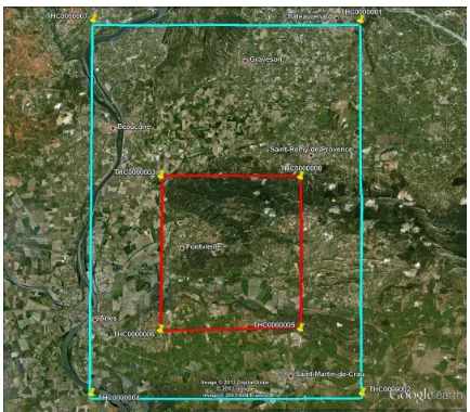
water bodies). The area used in this paper spans 4◦40’ to 4◦50’
E and 43◦39’ to 43◦46’ N (Figure 1(a)) and is about 100 Km2 .
The SAR data over Maussane test site was collected in 2009 and consists of orthorectified aerial SAR images (Figure 1(b)), DSM (Figure 1(c)) and DTM which were interferometrically produced, and the 3D road network (Figure 1(b)) which was extracted by the orthorectified SAR images and the DSM/DTM ((Mercer, 2007), (Zhang et al., 2010), www.intermap.com). The orthorectified SAR images have 1.25 m pixel size and according to the gen-eral accuracy specifications their horizontal absolute accuracy is 4 m (CE90%). The DSM/DTM are posted at 5 m and according to the general accuracy specifications the vertical accuracy is<1
m (LE90%) for the 40% of the coverage area, 1–3 m (LE90%) for the 40% of the coverage area and>3m (LE90%) for the rest 20% of the coverage area. The planar geometry of roads’ cen-trelines was extracted from the orthorectified SAR images and the elevation of the centrelines was determined from the interfer-ometrically produced DTM/DSM. The accuracy of the 3D road network meets the accuracy of the initial SAR data. The planar coordinates (geographic latitude/longitude) are available in the horizontal geodetic datum ETRS89 (European Terrestrial Refer-ence System 1989). The orthometric elevation is provided in the EGG07 (European Gravimetric Geoid model 2007) vertical geoid model.
The optical image was collected in 2010 and it is a level 2A standard satellite imagery. The nominal spatial resolution of the panchromatic imaging mode is 50 cm, and 2 m for the multispec-tral (8 specmultispec-tral bands) imaging mode (http://www.digitalglobe.com). The general geolocation accuracy specification of the optical im-age is 6.5m (CE90%), with predicted performance in the range of 4.6 to 10.7 m (CE90%), excluding terrain and off-nadir effects. The geolocation accuracy specification of the optical image using GCPs is 2.0 m CE90% (http://www.digitalglobe.com). The off-nadir view angle is36◦, the cross-track view angle is34.7◦and
the in-track view angle is−10.4◦for the specific image used in
this paper (Nowak Da Costa and Walczynska, 2011).
3 OVERVIEW AND OBJECTIVE
The general objectives of the study are: 1) to contribute to the evaluation of SAR data as source of GCI for the georeferenc-ing of optical images and 2) to benchmark the performance of two alternatives forms of GCI: Ground Control Linear Features (GCLFs) and Ground Control Points (GCPs). The accuracy of the georeferencing (either using GCLFs or GCPs) is computed using manually collected independent check points (CPs). The racy of the georeferencing is compared to the geolocation accu-racy specification of the optical image, as well as to the accuaccu-racy of the exhaustive georeferencing done by third parties. The test area is the well-known JRC’s Maussane test site near Mausanne-les-Alpilles in France.
The georeferencing process establishes the relationship of the 2D image space with the 3D object space. 3D-2D projection trans-formation models (empirical or physical) are used for this pur-pose (Toutin, 2004), (Dowman et al., 2012). Although literature abounds with fully justified conclusions on the general unsuitabil-ity of 2D-2D projective transformations for the georeferencing process, 2D-2D transformations (even simple 2D rigid and affine ones) are still used for the development of methods for the co-registration of optical and SAR images. Arbitrary assumptions such as of flat terrain, small image patches and geometrically cor-rected images, enable such methods to compute good results.
The objective of this paper is to test the performance of the 2D-2D projective transformations applied to the georeferencing of a
(a) Test site and coverage of the satellite optical image(in red) and the aerial SAR data (in cyan)
(b) 3D roads centrelines overlaid on the orthorectified SAR image
(c) The interferometrically produced DSM
level 2A satellite optical image using SAR data (in other words the co-registration of optical and SAR data), over greater areas of Earth’s surface (not just small image patches), with terrain of arbitrary form (not necessarily flat). Two different transformation models are used in this paper: 1) 2D-2D and 2) 3D-2D 1st order polynomial functions (PFs). Two different forms of GCI are used: 1) GCPs and 2) GCLFs.
4 METHOD
The significance of using GCI for the geometric correction of op-tical images has been noted, analyzed, researched and discussed exhaustively in the related literature. The most common form of GCI is the point, the fundamental feature of all photogrammet-ric processes. Numerous methods, data sets and tests have been presented over the years using GCPs ((Toutin, 2004), (Dowman et al., 2012). Repetition of this long-term research and practical knowledge would be redundant.
More complex features, such as straight lines and free form linear features can be exploited as an alternative/complementary form of GCI. The use of these features is not common (research is still in progress and the only software available is in-house de-veloped research software). In this paper, the use of GCLFs is based on the matching method introduced in (Vassilaki et al., 2008). The iterative closest point (ICP) algorithm ((Besl and McKay, 1992), (Zhang, 1994)) is used for accurate and robust global matching of heterogeneous FFLFs. The method matches 2D heterogeneous FFLFs with a rigid transformation. It was further expanded in order to match FFLFs of different dimen-sionality (3D-2D) with non-rigid projective transformation and it is fully documented in (Vassilaki et al., 2012b). For efficiency convenience and user friendliness the method has been incor-porated into ThanCAD (Stamos, 2007), an open-source CAD (http://sourceforge.net/projects/thancad/).
The matching of two FFLFs of the same dimensionality (2D-2D, 3D-3D) is done by an iterative process of determining closest point pairs between the two FFLFS and then using them to com-pute the transformation parameters by least squares adjustment (LSA). Closest point pairs are computed by splitting a FFLF to a large set of consecutive interpolated points, each one very close to its previous and its next point. Then, the distances of all these points to a node of the other FFLF are computed; the closest points between the two FFLFs are the points with the smallest dis-tances. This process may be computationally expensive but it is doable with modern computers, and it is relatively easy to speed it up with a divide-and-conquer approach. Further acceleration can be achieved by parallel computing (Stamos et al., 2009). In the case of FFLFs of different dimensionality (3D-2D) the 3D nodes of the 3D FFLF are projected to the 2D image space using an ini-tial or previous approximation of the transformation parameters, saving the association of each 3D node and its 2D projection. The closest points computed as in the 2D-2D case, are converted to 3D-2D pairs through the saved association, and they are used to compute the projection parameters by LSA.
The ICP algorithm needs a good initial approximation to con-verge, which means that the two FFLFs must be close enough to each other. Automatic pre-alignment is done using the rigid similarity transformation computed exploiting physical proper-ties of the two FFLFs, or using the non-rigid first order poly-nomial (affine) transformation computed exploiting characteristic statistical properties of the FFLFs (Vassilaki et al., 2012b).
In the case of networks of FFLFs of the same dimensionality (2D-2D, 3D-3D) or different dimensionality (3D-2D), the cor-respondences of FFLFs must be established. Assuming that the
two data sets are initially pre-aligned, a FFLF of the first data set corresponds to the FFLF of the other data set which is ‘clos-est’ to it. However, the definition of ‘clos‘clos-est’ is ambiguous for a FFLF which may span many other FFLFs. Different nodes of the same FFLF may be closest to nodes of different FFLFs. (Vassilaki et al., 2009a) introduced the term ‘distance’ as an in-tegral measure of how far or how different two FFLFs are. The pair of FFLFs which have the smallest ‘distance’ are assumed to correspond to each other. Four candidates for the ‘distance’ measure were suggested: the Euclidean distance between charac-teristic homologous points, namely the first nodes (d1), the last nodes (dN), or the centroids (d), and the absolute difference of the FFLFs lengths (S). For robustness, the biggest of these four values can be used as the ‘distance’ of the FFLFs. In the very unlikely case that the ‘distance’ is ambiguous (almost the same) for two or more pairs of FFLFs, application of the full ICP can be used to determine which FFLFs correspond to each other. ICP is the best and more robust approach, but it is very time con-suming and should be avoided if possible. The method proceeds with an ICP step, it brings the FFLFs even closer and it then re-evaluates the correspondence, as the ”distance” between any pair of FFLFs is obviously changed. Furthermore, ICP automatically rejects two unrelated FFLFs marked to correspond if they do not overlap (Vassilaki, 2012a).
All the FFLFs of a network share a common transformation. In order to compute the common transformation, LSA is applied to all the pairs of FFLFs simultaneously. The equations produced by the homologous points of all pairs of FFLFs are assembled into the same LSA matrices. The LSA computes the transformation which best fits all the pairs of FFLFs. The computed transfor-mation brings the FFLFs closer together, and thus the correspon-dences are re-evaluated, in case that the previous, poorer, trans-formation led to a few false correspondences. Since all pairs of FFLFs share the same transformation, a good approximation of the transformation of a single pair of FFLFs, automatically com-puted ((Vassilaki, 2012a), can be used to bring the data sets close together, essentially prealigning them.
5 APPLICATION AND RESULTS 5.1 Measurement of the GCI
160 common points were identified between the optical and the SAR image. They were measured in the 2D optical image space (pixels) and in the 3D object space (meters) of the SAR im-age. The elevation of the points measured on the SAR image was interpolated from the available interferometrically produced DEM (DSM). Some of the points were used as GCPs in order to compute the transformation models, and the remainder of the points were used as CPs in order to evaluate the computation. As the optical and the SAR image were unitemporal and the SAR image was orthorectified, it was not very hard to identify com-mon regions and characteristics. On the other hand, the fuzzy and speckled nature of the SAR image made the identification and measurement of single points ambiguous. The computation of the transformation model (Section 5.2) and its application to project 3D points to the optical image, revealed a few gross er-rors and point ambiguities, which either could not be resolved and thus new points were measured, or led to re-measurement of the picked points. The procedure was then iterated many times. In general the measurement of the common points between the optical and the SAR image was a very laborious process.
of the centrelines of the roads (3D Road Vectors) (Zhang et al., 2010) and thus no extraction of roads was necessary on the SAR data (Figure 1(b)). Common roads between the SAR data and the optical image were identified and then the edges of the roads were extracted manually on the optical image. The centrelines of the roads on the optical image space were computed with skele-tonization techniques. Although it was possible to identify a mul-titude of common roads between the optical and the SAR image, just a few of them were sufficient to ensure full GCI coverage of the optical image. The road centrelines were then used as match-ing primitives. The FFLFs with known 2D optical image space coordinates and known 3D object space node coordinates (read-ily available from the orthorectified SAR image and the DEM) were then used as GCLFs in order to compute the transformation model. Some editing (mostly merging) was needed to group the 3D roads according to the 2D roads. In general the measurement of common FFLFs was a straightforward and swift process.
5.2 Computation of the georeferencing
For both forms of GCI, 2D-2D and 3D-2D transformation mod-els were used to georeference the optical image. The transforma-tion models used are the following 1st order polynomial functransforma-tions (PFs):
- the 2D-2D 1st order PFs
x=a1X+a2Y +a3
y=b1X+b2Y +b3
(1)
- the 3D-2D 1st order PFs
x=a1X+a2Y +a3Z+a4
y=b1X+b2Y +b3Z+b4
(2)
Four combinations of GCI and transformation models were used for the computation of the georeferencing of the optical image: 1) 2D-2D PFs and GCPs
2) 2D-2D PFs and GCLFs 3) 3D-2D PFs and GCPs 4) 3D-2D PFs and GCLFs
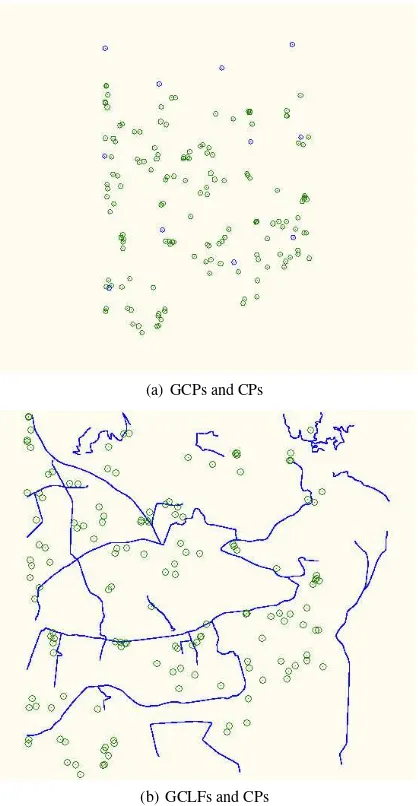
In the first and the third case 11 points which span the optical image were used as GCPs (Figure 2) for the computation of the correspondent transformation model. In the second and the fourth case 23 FFLFs which span the optical image were used as GCLFs (Figure 2) for the computation of the correspondent transforma-tion model. As a byproduct of the georeferencing process, the 23 GCLFS also produced automatically 91788 common 3D-2D points between the two data sets (2D optical image space and 3D object space of the SAR image). These points can be exploited by any standard photogrammetric/remote sensing software which does not have GCLFs capabilities.
5.3 Evaluation
The RMSE of the four cases was computed using manually col-lected independent CPs. From the 160 common points between the optical and the SAR image (Section 5.1), 11 points were used as GCPs (Section 5.2) and the remaining 149 points (in green in Figure 2) were used as CPs. The RMSE is shown in Table 1. The accuracy of the four cases was evaluated using:
1) the geolocation accuracy specification of the optical image which is 6.5 m (CE90%), with predicted performance in the range of 4.6 to 10.7 m (CE90%), excluding terrain and off-nadir effects. 2) the geolocation accuracy specification of the optical image with registration to GCPs which is 2.0 m (CE90%).
3) the accuracy computed independently by JRC using GCPs and CPs measured with GPS ((Nowak Da Costa and Walczynska,
(a) GCPs and CPs
(b) GCLFs and CPs
Figure 2: The distribution of the GCPs (in blue), the GCLFs (in blue) and the CPs (in green) over the test site.
2011)) and exhaustive testing of mathematical models as imple-mented in numerous standard software. The computed accuracy (Table 1) shows that:
1) The 2D-2D transformations lead to far worse accuracy (sev-eral tens of meters) than the geolocation accuracy specification defined by the operator of the sensor (6.5 m), for both forms of GCI (GCPs and GCLFs). Furthermore, since a level 2A satellite optical image was used in this paper, the accuracy is expected to be even worse in the case of basic imagery products (for instance level 1A). Thus the 2D transformations should be abandoned for real world practical cases over greater areas of Earth’s surface with arbitrary terrain.
2) The two forms of GCI (GCPs and GCLFs) used in this paper lead to the same accuracy (3.5 m), probably because it reflects the accuracy of the CPs themselves, namely 4 m planar and 1–2 m vertical accuracy. However, it should be noted that the
mea-Model GCI X (m) Y(m) Planar (m) 2D-2D PFs GCPs 32.3 14.6 35.4
GCLFs 37.8 35.0 51.5 3D-2D PFs GCPs 2.5 2.7 3.7
GCLFs 2.5 2.4 3.5
surement of the common points between the optical and the SAR image was a laborious process and thus the georeferencing using GCLFs is considered superior. 3) The computed accuracy (3.5 m) does not (and can not) meet the geolocation accuracy specifi-cation with registration to GCPs (2 m). More accurate GCI (for example measured with GPS) should be used for this purpose (Nowak Da Costa and Walczynska, 2011). However, the com-puted accuracy (3.5 m) is better than the geolocation accuracy specification without GCPs (6.5, with predicted performance in the range of 4.6 to 10.7 m), more so because the geolocation ac-curacy specification does not include terrain and off-nadir effects, while the test region and data include both effects.
6 CONCLUSION
In this paper the first results of an on-going study on the evalu-ation of SAR data as source of GCI, under realistic conditions, were presented. More specifically GCPs and GCLFs were col-lected from orthorectified SAR images and the corresponding in-terferometrically produced DEM. They were used to compute the georeferencing of a level 2A satellite optical image over a greater areas of Earth’s surface (not just a small patch), with arbitrary terrain type (not necessarily flat). Both 2D-2D and 3D-2D trans-formation models were used and the accuracy was evaluated us-ing independent CPs. The accuracy of the 2D-2D models was unacceptable to the point that they should not be used at all. The accuracy of the 3D-2D models reached the accuracy of the CPs themselves, which suggests that more accurate GCI will probably lead to better accuracy, and that SAR data has compatible accu-racy with optical images. Further research and experimentation on the subject is thus encouraged.
ACKNOWLEDGEMENTS
This research has been co-financed by the European Union (Eu-ropean Social Fund - ESF) and Greek national funds through the Operational Program ”Education and Lifelong Learning” of the National Strategic Reference Framework (NSRF) - Research Funding Program: Heracleitus II. Investing in knowledge society through the European Social Fund. The authors are also grate-ful to Dr Bryan Mercer of Intermap Technologies Inc. Intermap Technologies Inc. kindly provided the NEXTMap Europe SAR data (DSM, DTM, ORI and 3D Road Vectors). The WorldView-2 optical image ( cDigitalGlobe [2010], all rights reserved; pro-vided by European Space Imaging) is courtesy of the European Commission DG Joint Research Centre, Institute for the Protec-tion and Security of the Citizen, Community Image Data Portal of the Monitoring Agricultural Resources Unit. The authors are grateful to Dr Kay Simon and Lucau Cozmin.
REFERENCES
Besl, P.J. and McKay, N.D., 1992. A Method for Registration of 3-D Shapes. IEEE Transactions on Pattern Analysis and Machine Intelligence 14(2), pp. 239–256.
Dare, P. and Dowman, I., 2001. An improved model for automatic feature-based registration of SAR and SPOT images. ISPRS Jour-nal of Photogrammetry and Remote Sensing 56(1), pp. 3–28.
Dowman, I., Jacobsen, K., Konecny, G. and Sandau, R., 2012. High Resolution Optical Satellite Imagery. Whittles Publishing.
Hong, T.D. and Schowengerdt, R.A., 2005. A Robust Tech-nique for Precise Registration of Radar and Optical Satellite Im-ages. Photogrammetric Engineering and Remote Sensing, 71(5), pp. 585–593.
Karjalainen, M., 2007. Geocoding of synthetic aperture radar images using digital vector maps. IEEE Geoscience and Remote Sensing Letters, 4 (4), pp. 616–620.
Mercer, B., 2007. National and regional scale DEMs created from airborne InSAR. International Archives of Photogrammetry, Remote Sensing and Spatial Information Sciences, 36(3/W49B), pp. 113–117.
Nowak Da Costa, J.K. and Walczynska, A., 2011. Geometric Quality Testing of the WorldView-2 Image Data Acquired over the JRC Maussane Test Site using ERDAS LPS, PCI Geomatics and Keystone digital photogrammetry software packages - Initial Findings with ANNEX. European Commission, Joint Research Centre, Institute for Environment and Sustainability, JRC 64624.
Reinartz, P., Mueller, R., Schwind, P., Suri, S. and Bamler, R., 2011. Orthorectification of VHR optical satellite data exploiting the geometric accuracy of TerraSAR-X data. ISPRS Journal of Photogrammetry and Remote Sensing, 66(1), pp. 124–132.
Stamos, A.A., 2007. ThanCad: a 2dimensional CAD for engi-neers. Proceedings of the Europython2007 Conference, Vilnius, Lithuania.
Stamos, A.A., Vassilaki D.I. and Ioannidis, Ch.C., 2009. Speed Enhancement of Free-form Curve Matching with Parallel Fortran 2008. in B.H.V. Topping, P. Ivnyi, (Editors), Proceedings of the First International Conference on Parallel, Distributed and Grid Computing for Engineering, Civil-Comp Press, UK.
Toutin, T., 2004. Review Paper: Geometric processing of remote sensing images: models, algorithms and methods. International Journal of Remote Sensing, 25(10), pp. 1893–1924.
Vassilaki, D.I., Ioannidis, C. and Stamos, A.A., 2008. Regis-tration of 2D Free-Form Curves Extracted from High Resolu-tion Imagery using Iterative Closest Point Algorithm. EARSeL’s Workshop on Remote Sensing - New Challenges of High Reso-lution, Bochum, Germany pp. 141–152.
Vassilaki, D.I., Ioannidis, C. and Stamos, A.A., 2009. Multitem-poral Data Registration through Global Matching of Networks of Free-form Curves. FIG Working: Surveyors Key Role in Accel-erated Development, May 3-8, Eilat, Israel.
Vassilaki, D.I., Ioannidis, C. and Stamos, A.A., 2009. Registra-tion of Unrectified Optical and SAR imagery over Mountainous Areas through Automatic Free-form Features Global Matching. International Archives of Photogrammetry, Remote Sensing and Spatial Information Sciences, 36(1-4-7/W5).
Vassilaki, D.I., Ioannidis, C. and Stamos, A.A., 2011. Georefer-ence of TerraSAR-X images using sciGeorefer-ence orbit data. EARSeL Symposium Proceeding: Remote Sensing and Geoinformation not only for Scientific Cooperation in Prague, Czech Rebublic, May 30 – June 2, pp. 472–480.
Vassilaki, D.I., 2012. Matching and evaluating free-form linear features for georeferencing spaceborne SAR imagery. Photogrammetrie, Fernerkundung, Geoinformation, 2012(4), pp. 409–420.
Vassilaki, D.I., Ioannidis, C. and Stamos, A.A., 2012. Automatic ICP-Based Global Matching of Free-Form Linear Features. The Photogrammetric Record, 27(139), pp. 311–329.
Zhang, Z., 1994. Iterative Point Matching for Registration of Free-form Curves and Surfaces. International Journal of Com-puter Vision 13(2), pp. 119–152.