Integrating model knowledge into SVM classification – Fusing hyperspectral and laserscanning data by kernel composition
Andreas Ch. Braun, Uwe Weidner, Boris Jutzi, Stefan Hinz
KEY WORDS:hyperspectral, airborne laserscanning, data fusion, support vector machine, kernel composition
1 INTRODUCTION
Roof materials are important sources of pollutants within cities. To monitor and quantify polluted roof runoff, a precise classifica-tion approach of various roof material classes is needed. Within urban environments, different geometries of roofs exist, e.g. sloped roofs and flat roofs, which can be distinguished by using ALS data. To precisely classify different roof material classes, e.g. brick, slate, gravel, hyperspectral datasets can be utilized. Thus, exploitation of both hyperspectral and ALS data is helpful. In order to exploit these data sources, data fusion needs to be performed. A novel approach for data fusion is possible with kernel composition methods. Support vector machines (SVMs) have proven to be capable classifiers for hyperspectral and ALS data separately, but also for combined datasets [Camps-Valls et al., 2006]. Kernel functions are used to find the solutions of SVM classifiers. The kernel composition [Camps-Valls et al., 2006] takes account of the fact, that kernel functions can be combined (e.g. by addition) to form new kernels. This combination offers a novel option for data fusion. An application for the fusion and classification of hyperspectral and ALS data is given in [Braun et al., 2011].
SVMs are binary classifiers. To classify n classes (with n > 2), strategies have to be employed which break down the n class case to various two class cases. The one-against-one strategy considers only two of the n classes at each step. This feature is exploited herein to selectively use the ALS data when needed. Thus, incorporating model knowledge on the roof geometry into the classification process is made possible.
The remainder of the paper is organized as follows. Sec-tion 2 presents a mathematical introducSec-tion into the methods used. Theν-SVM by [Schoelkopf et al., 2001] is introduced. Afterwards, two data fusion approaches –concatenation and ker-nel composition– are introduced. Finally, the One-Against-One cascade is explained with special emphasis on its usage for class dependent data fusion. Section 3 outlines the data preprocessing employed herein. In section 4 classification results based on both data fusion approaches are presented and compared. Some considerations and evaluations on the approach followed are given. Finally, section 5 concludes the work presented and gives an outline on further investigations.
2 MATHEMATICAL FOUNDATIONS
This section presents brief mathematical foundations on the methods employed. Kernel composition makes use of the fact that kernels can be combined by arithmetical operations like ad-dition or multiplication. By accepting a small amount of falsely classifed training data, SVMs ensure appropriate generalization. The strategy most frequently used for error handling is the Cost-SVM [Cortes and Vapnik, 1995]. In this paper, emphasis is put on a different error handling strategy calledν-SVM [Schoelkopf et al., 2000]. Due to the fact that one of its parameters can be ad-justed to decribe the amount of noise within the training datasets, it has advantages overCost-SVM.
2.1 ν-SVM with linear kernel
ν-SVM is used to separate different classes from one another. For a training data setXset withlsamplesxi, each sample has a class labelyi∈ {−1,+1}which assigns it to one of two classes. ν-SVM now finds a subsetSV ⊂ Xof samplesxi, which are closest to the samples of the respective other class. The samples of this subset are called support vectors. They are used to con-struct a separating plane which sections the members of class +1 from class -1. The method chooses the samples which allow best for a trade-off between correctly separating the two classes and leaving a maximum margin between the classes for generaliza-tion. To simplify finding this trade-off, small errors (samples that are on the wrong side of the plane) are allowed by slack variables ξi.
Note that Eq.1 is very similar toCost-SVM (cf. [Burges, 1998]), however, the regularization constant ν is not unbounded, but ν ∈(0,1]. The parameterνdescribes to which extent the train-ing data are affected by noise. Note that in Eq.1&2, the original dataxiare used to find a separating plane – the originallinear for-mulation of the SVM is used [Cortes and Vapnik, 1995], [Burges, 1998]. However, it may not always be possible to find a linear so-lution in the original data space. Hence, usually data are mapped into a higher-dimensional space by non-linear feature functions Φ(xi). In this case, the constraint given by Eq.2 would change to:
subject to yi((w·Φ(xi)) +b)≥ρ−ξi (3)
ξi≥0, ρ≥0
All types of SVMs obviate calculatingΦ(xi)by introducing ker-nels (cf. Eq.4) to avoid computational cost. Thus, the kernel function induces a high dimensional reproducing kernel Hilbert space (RKHS), making the problem linearly solvable within this high dimensional space. The radial basis function is the kernel function most frequently used when linearity of the separation problem can not be assumed in the original data space [Keerthi and Lin, 2003], [Melgani and Bruzzone, 2004], [Huang et al., 2002]. Within this paper, the linear kernel is used though. It rep-resents a dot product of the features (cf. Eq.4) and thus, doesnot induce a high dimensional RKHS. The reason for using the linear kernel is that over one hundred hyperspectral channels and fur-thermore multiple features derived from the ALS data are avail-able. Furthermore, as the one-against-one strategy considers only two classes in one step, leading to an inherently sparse feature space. Hence, utilizing a linear kernel seems sufficient. As the classification problem is simplified, it can be considered as lin-early solvable in the first place.
2.2 Approaches for Data Fusion
concate-nation and kernel composition – a data fusion approach available for kernel based classifiers like SVMs.
Concatenation When fusing information from two different sensors, like hyperspectral data and ALS data in this case, the most simple approach is to concatenate the two data matrices to a single matrix. However, given over one hundred spectral chan-nels of HyMap and only a few information chanchan-nels derived from the ALS data one can not be sure whether the geometric informa-tion is utilized adequately by the classifier or whether the multi-tude of spectral channels and their noise outweigh the informa-tion of the ALS data.
Kernel Composition Kernel matrices computed through ker-nel functions are the representation of the input data used to iden-tify the support vectors. The kernel function originally proposed in [Cortes and Vapnik, 1995] is the linear kernel, a dot product between two points from the training data set. Givenltraining points, all possiblel2 dot products of two pointsxiandxjare
computed, resulting in anl×lkernel matrixKi,j (cf. Eq.4). According to Mercers theorem [Mercer, 1909], kernel matrices can be combined by certain arithmetical operations like addition, multiplication etc. Hence, data fusion can be performed by com-puting one kernel on the spectral domain and another kernel on the geometric domain. Afterwards, they are added to perform data fusion (cf. Eq.6).
Kcomposite=λ1Kspectral+λ2Kgeometric (6)
λ1∈(0,1], λ2= 1−λ1
Note that through tuningλ1andλ2, the user can define to which
extent the information in each domain is considered as significant for the classification problem. An option not available for simple concatenation of the data when using SVM.
2.3 Exploitation of One-Against-One Cascade
SVMs are binary classifiers, they solve classification problems given two classes. Here, 14 subclasses need to be distinguished (cf. Tab.1). Hence, the 14-class problem needs to be broken down into several two class problems. The one-against-one stategy considers each 142permutation of the classes separately – which leads to 91 training and classification steps. At each step, a model is trained to distinguish two classes, considering e.g. the training pixels of class 6 from the training pixels from class 9. Within the classification step, this SVM would assign either 6 or 9 as a label to each pixel, although the majority of pixels should belong to classes different to six or nine. Thus, a considerable part of pixels will be falsely classified by this particular SVM. However, during classification, each pixel is labeled by all 91 models. Hence, each pixels receives 91 labels dwithd∈[1, . . . ,14]. A1×91label vectorvifor each pixels is produced. The class membership for theith pixel is decided bymod(vi)the label most frequently assigned to the pixel (Max Wins strategy). The Max Wins strategy allows for a robust classification although each pixel is assigned falsely by some of the 91 SVMs.
As mentioned above, two different types of roof geome-tries are of interrest in the ALS dataset – sloped roofs and flat roofs. While information of the ALS data can be helpful to distinguish between sloped brick roofs and flat gravel roofs, it should not faciliate the separation of e.g. sloped brick roofs and sloped slate roofs. As the one-against-one strategy does not consider all 14 classes in one step, the cascade can be exploited to recognize whether the user considers geometry as significant for each classification step. When separating two roof material classes with different geometries (sloped vs. flat) the spectral
domain is fused with the geometric domain by concatenation or kernel composition. In contrast, when separating similar roof geometries (sloped vs. sloped or flat vs. flat), the geometric domain is left out and the spectral domain is used exclusively. By this, data known for not containing any new information can be ommitted and training the classifier is better focused in a easy and straightforward manner. Hence, the model knowledge about the roof geometry can be brought into classification in a quick and straightforward manner.
3 DATAPREPARATION ANDCLASSES
An image from the city of Karlsruhe, taken by the HyMap sensor in 2003 with a spatial resolution of 4×4 m provides the hyper-spectral information. A laserscan with 1×1 m resolution from 2002 delivers geometrical information. A building mask is de-rived from the first pulse information to indicate buildings and mask out other objects which do not relate to roofs. The mask is required as all classification approaches implemented here are relative SVM approaches. Thus, they have the disadvantage of also assigning non-building areas –like vegetation or roads– to roof material classes if there classes are not assigned as training classes, [Braun, 2010], [Braun et al., 2011]. After classification, the mask will be used to assign these areas to the rejection class.
3.1 Data Preprocessing
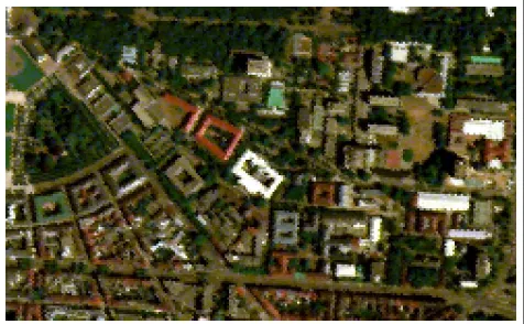
The data of HyMap is resampled to the spatial resolution of the laser scan, using nearest neighborhood. To reduce computational cost, and to allow for a later comparison with [Lemp and Wei-dner, 2004] and [Braun et al., 2011], a 605×987 pixel subset is chosen which shows the campus of KIT (cf. Fig.1, & Fig.2). Az-transformation (i.e. normalization by mean and standard deviation) on each layer is performed to ensure comparability. A mean-shift segmentation on the first pulse information is per-formed as entire roof segments have to be classified. Apart from the first pulse and last pulse information, the gradient and curva-ture of the first pulse and are computed. This information is used to distinguish sloped roofs from flat roofs. Hence, six informa-tion channels are derived from the ALS data. In addiinforma-tion, 126 hyperspectral channels are available, resulting in a feature space with 132 features.
3.2 Classes of roof materials
Training areas for different roof material classes are assigned. To ensure comparability with the results already obtained at IPF, the same classes as in [Lemp and Weidner, 2004] and [Braun et al., 2011] are defined and training areas for them are assigned. In [Braun et al., 2011] for each roof material class, only one training class is assigned. However, this could lead to unnecessar-ily complicated separation problems as incorporating e.g. bright, newly tiled brick roofs and dark, weathered brick roofs into the same class spreads out this class significantly within the feature space. This may cause overlap with other classes. Hence,
like in [Braun et al., 2011], each roof material class is divided into several subclasses. After classification, these subclasses are agglomerated into the final roof material classes. In Tab.1 the roof material classes and their colors in the classification results are indicated. nSC indicates the number of subclasses for the respective roof material class.
Table 1: Roof Material Classes
Roof Class Abbr. Geometry nSC Color Pollutant
Brick C1 sloped 3 PAC
Copper C2 sloped 2 Cu/PAC
Gravel C3 flat 2 PAC
Slate C4 sloped 2 —
Zinc C5 flat 3 Zn/PAC
Stone-like C6 flat 2 PAC
3.3 Data Fusion and Training
For each training class the spectral and geometric information in the two domains is derived. Several preliminary and final classi-fication approaches are carried through. The first one to be em-phasized here is fusing the information by concatenation. For the second, one kernel for each of the two domains is calculated and used for kernel composition to obtain a new kernel as explained in subsection 2.2. The parameterνis for error handling as it re-lates to the amount of noise in the training data. As only a small amount of noise is expected,ν = 0.05is chosen. Both training and classification are accomplished, using LibSVM 2.91 [Chang and Lin, 2001] for Matlab.
4 RESULTS AND DISCUSSION
At first, a thourough comparison between the classification meth-ods used and alternatives are given. Thus, the main assumptions are evaluated and a final classification strategy is developed. Af-terwards, a comparison between two data fusion approaches, fol-lowed by classification usingν-SVM is presented. At first, data fusion is performed by simple concatenation. Secondly, kernel composition is performed for data fusion. Both approaches ex-ploit the one-against-one cascade to use the information of the ALS data only for separation between roof material classes with different geometry (i.e. sloped vs. flat).
4.1 Validity of the Approach
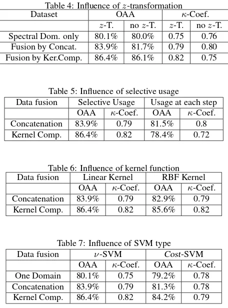
The approach constitutes some major assumptions. The first one is that ALS data is needed to distinguish the roof material classes. To prove this, a test on the counter hypotheses is per-formed by classifying the dataset using only the hyperspectral information [Lemp and Weidner, 2004]. As Tab.4 reveals, the accuracies yielded using only the spectral information are lower
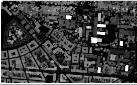
Figure 2: Visualization of First Pulse
than for using both hyperspectral and information of the ALS data. Hence, the assumption that ALS data should be exploited can be confirmed although the loss of accuracy when using the spectral domain exclusively is only moderate. An approach ex-plicitly based on hyperspectral data could also be followed with only a slight loss in accuracy. Secondly, the classification prob-lem is considered to be linear in the original feature space. An-other important assumption is that a linear kernel (cf. Eq.4) in-stead of an RBF kernel (cf. Eq.5) can be used. To validate this assumption, different classifications are carried through using an RBF kernel. The RBF kernels parameterσis optimized jointly withνusing 5-fold grid search. As Tab.6 reveals, both kernels produce comparable results. Thus, it is confirmed that the linear kernel can be used. Therefore, the second assumption of linearity in the original feature space due to its high dimensionality can be confirmed as well. Another assumption is, that performing az-transformation on the data contributes to higher classifica-tion accuracies. For each of the three classificaclassifica-tion approaches (using only the spectral domain, data fusion by concatenation and data fusion by kernel composition) classification is carried through both with and without priorz-transformation. A com-parison is given in Tab.4. As one can see, classification accu-racy for all approaches could by raised slightly through prior z-transformation. Hence, it can be confirmed thatz-transforming the data raises classification accuracy for the given dataset. Fur-thermore, it is assumed thatν-SVM [Schoelkopf et al., 2001] yields higher classification accuracies thanCost-SVM by [Cortes and Vapnik, 1995]. Again, a comparison for all approaches is car-ried through. As Tab.7 shows,ν-SVM indeed yields higher ac-curacies for all approaches. This finding is especially interesting, as forCost-SVM, the parameterC– which can not be estimated directly – is optimized by 5-fold cross validation search. In con-trast, the parameterνfor theν-SVM approach is simply set to 0.05. From there, theν-SVM approach is recommendable for the classification of the combined dataset (cf. Tab.4). The most im-portant assumption, however, is that the one-against-one cascade should be exploited to use the geometric informationselectively – i.e. when roof material classes with different geometry are to be separated– instead of using geometric information at each step. Again, a comparison between both usages is performed. The con-fusion matrices (cf. Tab. 5) reveal that selective usage yields higher accuracies, with a certain advantage for the data fusion approach based on kernel composition. Hence, it can be con-cluded that information of the ALS data should only be used for separation of roof material classes with different roof shapes, not for the separation of roof material classes with equal roof shapes. and that the one-against-one classification cascade of SVM is a suitable way of using this information selectively. An alterna-tive to the one-against-one cascade could be the directed acyclic graph SVM [Platt et al., 2000]. It uses the same SVM models as one-against-one but implements a graph based decision strat-egy. These result lead to the final classification strategy, decribed below:ν-SVM classification with a linear kernel on datasets pre-processed byz-transformation and information fused by concate-nation (see Sec.4.2) and kernel composition (see Sec.4.3). The latter promises the highest classification accuracy.
4.2 Result using Concatenation
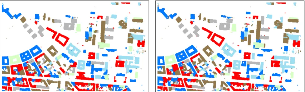
cam-Figure 3: Classification Result using Concatenation
paign is given in Tab.2∗. The overall accuracy is 83.9% and theκ
coefficient is 0.79. ClassC2:Copperis the class that yielded the lowest completeness (CP) and correctness (CR) values. The rea-son for these low values is confusion with classC1:Brick. Train-ing took 1.5 minutes and classification took 72 minutes. Hence, the classification phase being 48 times longer is much more im-portant under computational considerations, even when classify-ing only a small subset of the entire image.
4.3 Result using Kernel Composition
Fig.4 shows the classification result after kernel composition. Af-ter classifiacation, non-building areas are masked out again. The result is convincing in the major part of the image. As for the result of concatenation, some misclassifications occur due to roof structures e.g. made of metal within an area of slate or brick tiles. Again, a confusion matrix, calculated on the basis of control ar-eas assigned during a field campaign is given in Tab.31. The overall accuracy is 86.4% and theκcoefficient is 0.82. Hence, the accuracy values yielded are higher for the kernel compo-sition approach. Especially, for the classC2:Copper consider-ably higher values of completeness and correctness are yielded. There is much less confusion with the classC1:Brick. Also for the other classes, equal or even higher completeness and correct-ness values are achieved. At this point, however, these results should not be over interpreted but confirmed by further research efforts. As one can see, the visual results yielded by both data fusion approaches are quite similar. In Fig.5, green segments re-fer to buildings where both approaches assigned the same class, while red segments mark buildings for which the approaches dis-agree. Considering computational time, the kernel composition approach has advantages. Training took 0.7 minutes and classi-fication took 59 minutes. Hence, training is twice as fast than for data fusion by concatenation. As the time for training is very
∗OAA: overall accuracy,κ: kappa coefficient, CP: completeness, CR:
correct-ness
Table 2: Confusion Matrix forν-SVM after Concatenation
Control
C1 C2 C3 C4 C5 C6 CR
Classification
C1 18040 712 0 0 55 0 95.9
C2 0 2591 0 1804 0 0 58.9
C3 371 98 6216 2705 121 0 65.3 C4 1322 0 0 22439 2428 0 85.6
C5 0 0 0 441 18007 0 97.6
C6 0 39 939 1613 324 3569 55.0 CP 91.4 75.3 86.8 77.3 86.0 100 OAA 83.9
κ 0.79
Figure 4: Classification Result using Kernel Composition
short for both approaches, this advantage in computational ef-ficiency is neglectable. However, the classification procedure is around 13 minutes (∼18% less computation time) shorter for ker-nel composition. Keeping in mind, that the subset used here is only a small subset of the entire scene and that classification time scales linearly with the number of point to be classified, an as-sessment of the entire scene would be significantly shorter using kernel composition. The approach constitutes an improvement to [Braun et al., 2011] as the overall accuracy could be risen from 70.5% in [Braun et al., 2011] to 86.4% within this report. As the influence of the kernel function does not explain a significant increase in accuracy (cf. Tab.6) it has to be concluded that the increase of accuracy is explained by the splitting into subclasses. In contrast to [Braun et al., 2011], the roof material classes are split into subclasses. By doing so, the spreading of the classes within the feature space is reduced thus faciliating the separation process. It has to be assumed that splitting the classes explains the most for the higher classification accuracies.
5 CONCLUSIONS AND FUTURE WORK
Hyperspectral and ALS data are used jointly to classify an urban dataset into six roof material classes. A comparison for different data fusion approaches is presented. The classifier mainly used is theν-SVM proposed by [Schoelkopf et al., 2001]. In the first place, no data fusion is performed, but the hyperspectral data is classified exclusively. The classification accuracies yielded are lower than for the approaches using both hyperspectral and in-formation of the ALS data – as could be expected. However, the loss of accuracy which results from using only hyperspectral data is only a few percent points. This indicates that approaches exploiting the precise spectral information of the hyperspectral dataset without ALS data are also feasible. A more significant loss of classification accuracy has to be expected when using mul-tispectral data, which – unlike hyperspectral data – is not able
Table 3: Confusion Matrix forν-SVM after Kernel Composition
Control
C1 C2 C3 C4 C5 C6 CR
Classification
C1 18040 0 0 0 55 0 99.6
C2 0 3303 0 888 0 0 78.8
C3 371 98 6825 2705 121 0 67.4 C4 1322 0 0 23215 2428 0 86.0
C5 0 0 0 441 18007 0 97.6
C6 0 39 330 1753 324 3569 59.3 CP 91.4 96.0 95.3 80.0 86.0 100 OAA 86.4
to compensate the lack of geometric information by high spec-tral precision. For instance, one would not expect slate roofs and gravel roofs to be distinguished in a multispectral dataset without using further information. Before classification, data are standardized byz-transformation. The overall accuracy yielded on z-transformed data is higher than the one yielded on non-standardized data. Due to the high dimensionality of the origi-nal feature space (126 hyperspectral channels plus 6 information layers derived from laserscanning) the classification problem is assumed to be linearly solvable in the first place. Hence, a linear kernel instead of an RBF kernel is used. A comparison reveals that this assumption is justified as the accuracies yielded are com-parable for both kernels. Theν-SVM proposed by [Schoelkopf et al., 2001] instead of the Cost-SVM by [Cortes and Vapnik, 1995] is used. A comparsion attests higher classification accura-cies to theν-SVM. Two data fusion approaches –concatenation and kernel composition– are compared. The latter constitutes an approach specialized on SVMs. It yields higher classification ac-curacies than concatenation, especially for the classC2:Copper. To clarify the reasons of the advantage on this class, more re-search efforts need to be made on different datasets. The differ-ence in overall accuracy is 2.5 percent points. As an approach us-ing only hyperspectral information is feasible as well, ALS data is not indispensable for the given dataset. It has to be assumed that the differences between the two data fusion approaches should be more pronounced for datasets and classification problems which strictly require both information domains. However, the approach using kernel composition is significantly faster in classification and equal or better in precision than the result based on concate-nation. The information on roof geometry is not significant for all classification steps. The one-against-one cascade allows to use the geometric domain only for the steps where it is strictly needed. For the separation of roof material classes with sim-ilar geometry, this information can be omitted. A comparison between using ALS data at each step and using ALS data se-lectively yields higher accuracies for the latter. The information on geometry can therefore be used selectively. This allows the
Table 4: Influence ofz-transformation
Dataset OAA κ-Coef.
z-T. noz-T. z-T. noz-T. Spectral Dom. only 80.1% 80.0% 0.75 0.76
Fusion by Concat. 83.9% 81.7% 0.79 0.80 Fusion by Ker.Comp. 86.4% 86.1% 0.82 0.75
Table 5: Influence of selective usage
Data fusion Selective Usage Usage at each step OAA κ-Coef. OAA κ-Coef. Concatenation 83.9% 0.79 81.5% 0.8 Kernel Comp. 86.4% 0.82 78.4% 0.72
Table 6: Influence of kernel function Data fusion Linear Kernel RBF Kernel
OAA κ-Coef. OAA κ-Coef. Concatenation 83.9% 0.79 82.9% 0.79 Kernel Comp. 86.4% 0.82 85.6% 0.82
Table 7: Influence of SVM type
Data fusion ν-SVM Cost-SVM
OAA κ-Coef. OAA κ-Coef. One Domain 80.1% 0.75 79.2% 0.78 Concatenation 83.9% 0.79 81.3% 0.78 Kernel Comp. 86.4% 0.82 84.2% 0.79
Figure 5: Agreement of datafusion approaches. Green: same class label assigned, Red: different class labels assigned
user to bring in model knowledge into the pattern recognition ap-proach. Although the model knowledge is simply structured in this approach – it consists only in the decision whether a roof is sloped or flat – more complex knowledge is also usable with is approach. In the future, this approach will be extended to graph-based SVMs [Platt et al., 2000] and use the methodology on dif-ferent datasets. Furthermore, the advantages of difdif-ferent types of kernel composition (e.g. multiplication instead of addition) will be explored and compared.
REFERENCES
Braun, A., 2010. Evaluation of One-class SVM for Pixel-based and Segment-based Classification in Remote Sensing. In: Inter-national Archives of the Photogrammetry, Remote Sensing and Spatial Information Sciences, Vol. XXXVIII (Part 3B).
Braun, A., Weidner, U. and Hinz, S., 2011. Classifying Roof Materials using Data Fusion through Kernel Composition - Com-paringν-SVM and One-class SVM. In: In Proceedings: JURSE, Joint Urban Remote Sensing Event, Munich.
Burges, C., 1998. A tutorial on support vector machines for pat-tern recognition. Data mining and knowledge discovery 2(2), pp. 121–167.
Camps-Valls, G., Gomez-Chova, L., Mu˜noz-Mar´ı, J., Vila-Franc´es, J. and Calpe-Maravilla, J., 2006. Composite kernels for hyperspectral image classification. Geoscience and Remote Sensing Letters, IEEE 3(1), pp. 93–97.
Chang, C. and Lin, C., 2001. LIBSVM: a library for support vector machines.
Cocks, T., Jenssen, R., Stewart, A., Wilson, I. and Shields, T., 1998. The HyMapTM airborne hyperspectral sensor: the system, calibration and performance. In: Proceedings of the 1st EARSeL workshop on Imaging Spectroscopy, pp. 37–42.
Cortes, C. and Vapnik, V., 1995. Support-vector networks. Ma-chine learning 20(3), pp. 273–297.
Huang, C., Davis, L. and Townshend, J., 2002. An assessment of support vector machines for land cover classification. Interna-tional Journal of Remote Sensing 23(4), pp. 725–749.
Keerthi, S. and Lin, C., 2003. Asymptotic behaviors of sup-port vector machines with Gaussian kernel. Neural computation 15(7), pp. 1667–1689.
Lemp, D. and Weidner, U., 2004. Use of hyperspectral and laser scanning data for the characterization of surfaces in urban areas. In: XXth ISPRS Congress.
Mercer, J., 1909. Functions of positive and negative type, and their connection with the theory of integral equations. Philosoph-ical Transactions of the Royal Society of London. Series A, Con-taining Papers of a Mathematical or Physical Character 209(441-458), pp. 415.
Platt, J., Cristianini, N. and Shawe-Taylor, J., 2000. Large margin DAGs for multiclass classification. Advances in neural informa-tion processing systems 12(3), pp. 547–553.
Schoelkopf, B., Platt, J., Shawe-Taylor, J., Smola, A. and Williamson, R., 2001. Estimating the support of a high-dimensional distribution. Neural computation 13(7), pp. 1443– 1471.