in PROBABILITY
EXPLICIT BOUNDS FOR THE APPROXIMATION
ER-ROR IN BENFORD’S LAW
LUTZ D ¨UMBGEN1
Institute of Mathematical Statistics and Actuarial Science, University of Berne, Alpenegg-strasse 22, CH-3012 Switzerland
email: [email protected]
CHRISTOPH LEUENBERGER
Ecole d’ing´enieurs de Fribourg, Boulevard de P´erolles 80, CH-1700 Fribourg, Switzerland email: [email protected]
Submitted September 20, 2007, accepted in final form February 1, 2008 AMS 2000 Subject classification: 60E15, 60F99
Keywords: Hermite polynomials, Gumbel distribution, Kuiper distance, normal distribution, total variation, uniform distribution, Weibull distribution
Abstract
Benford’s law states that for many random variablesX >0 its leading digitD=D(X) satisfies approximately the equationP(D=d) = log10(1 + 1/d) ford= 1,2, . . . ,9. This phenomenon follows from another, maybe more intuitive fact, applied to Y := log10X: For many real
random variablesY, the remainder U :=Y − ⌊Y⌋is approximately uniformly distributed on [0,1). The present paper provides new explicit bounds for the latter approximation in terms of the total variation of the density ofY or some derivative of it. These bounds are an interesting and powerful alternative to Fourier methods. As a by-product we obtain explicit bounds for the approximation error in Benford’s law.
1
Introduction
The First Digit Law is the empirical observation that in many tables of numerical data the leading significant digits are not uniformly distributed as one might suspect at first. The following law was first postulated by Simon Newcomb (1881):
Prob(leading digit =d) = log10(1 + 1/d)
ford= 1, . . . ,9. Since the rediscovery of this distribution by physicist Frank Benford (1938), an abundance of additional empirical evidence and various extensions have appeared, see Raimi (1976) and Hill (1995) for a review. Examples for “Benford’s law” are one-day returns on stock market indices, the population sizes of U.S. counties, or stream flow data (Miller and Nigrini 2007). An interesting application of this law is the detection of accounting fraud (see Nigrini,
1RESEARCH SUPPORTED BY SWISS NATIONAL SCIENCE FOUNDATION
1996). Numerous number sequences (e.g. Fibonacci’s sequence) are known to follow Benford’s law exactly, see Diaconis (1977), Knuth (1969) and Jolissaint (2005).
An elegant way to explain and extend Benford’s law is to consider a random variableX >0 and its expansion with integer base b≥2. That means,X =M ·bZ for some integerZ and some
numberM ∈[1, B), called the mantissa ofX. The latter may be written asM =P∞
i=0Di·b−i
with digits Di ∈ {0,1, . . . , b−1}. This expansion is unique if we require that Di 6=b−1 for
infinitely many indices i, and this entails thatD0≥1. Then theℓ+ 1 leading digits of X are
equal tod0, . . . , dℓ∈ {0,1, . . . , b−1}withd0≥1 if, and only if,
d ≤ M < d+b−ℓ with d :=
ℓ
X
i=0
di·b−i. (1)
In terms of Y := logb(X) and
U := Y − ⌊Y⌋ = logb(M)
one may express the probability of (1) as
P¡logb(d)≤U <log
b(d+b−ℓ)
¢
. (2)
If the distribution ofY is sufficiently “diffuse”, one would expect the distribution of U being approximately uniform on [0,1), so that (2) is approximately equal to
logb(d+b−ℓ)−logb(d) = logb(1 +b−ℓ/d).
Hill (1995) stated the problem of finding distributions satisfying Benford’s law exactly. Of course, a sufficient condition would be U being uniformly distributed on [0,1). Leemis et al. (2000) tested the conformance of several survival distributions to Benford’s law using com-puter simulations. The special case of exponentially distributed random variables was studied by Engel and Leuenberger (2003): Such random variables satisfy the first digit law only ap-proximatively, but precise estimates can be given; see also Miller and Nigrini (2006) for an alternative proof and extensions. Hill and Schuerger (2005) study the regularity of digits of random variables in detail.
In general, uniformity of U isn’t satisfied exactly but only approximately. Here is one typical result: Let Y =σYo for some random variableYo with Lebesgue density fo on the real line.
Then
sup
B∈Borel([0,1))
¯
¯P(U ∈B)−Leb(B) ¯
¯ → 0 asσ→ ∞.
This particular and similar results are typically derived via Fourier methods; see, for instance, Pinkham (1961) or Kontorovich and Miller (2005).
The purpose of the present paper is to study approximate uniformity of the remainder U in more detail. In particular we refine and extend an inequality of Pinkham (1961). Section 2 provides the density and distribution function ofU in case of the random variableY having Lebesgue density f. In case off having finite total variation or, alternatively, f beingk≥1 times differentiable withk-th derivative having finite total variation, the deviation ofL(U) (i.e. the distribution of U) from Unif[0,1) may be bounded explicitly in several ways. Since any density may be approximated inL1(R) by densities with finite total variation, our approach is
2
On the distribution of the remainder
U
Throughout this section we assume thatY is a real random variable with c.d.f.Fand Lebesgue densityf.
2.1
The c.d.f. and density of
U
For any Borel setB⊂[0,1),
P(U ∈B) = X
z∈Z
P(Y ∈z+B).
This entails that the c.d.f.GofU is given by
G(x) :=P(U ≤x) = X
z∈Z
(F(z+x)−F(z)) for 0≤x≤1.
The corresponding densityg is given by
g(x) := X
z∈Z
f(z+x).
Note that the latter equation defines a periodic functiong :R→[0,∞], i.e.g(x+z) =g(x) for arbitraryx∈Randz∈Z. Strictly speaking, a density ofU is given by 1{0≤x <1}g(x).
2.2
Total variation of functions
Let us recall the definition of total variation (cf. Royden 1988, Chapter 5): For any interval J⊂Rand a functionh:J→R, the total variation ofhonJ is defined as
TV(h,J) := supn
m
X
i=1
¯
¯h(ti)−h(ti−1)
¯
¯ : m∈N; t0<· · ·< tm;t0, . . . , tm∈J
o
.
In case ofJ=Rwe just write TV(h) := TV(h,R). Ifhis absolutely continuous with derivative h′ inL1
loc(R), then
TV(h) =
Z
R| h′(x)
|dx.
An important special case are unimodal probability densities f on the real line, i.e.f is non-decreasing on (−∞, µ] and non-increasing on [µ,∞) for some real numberµ. Here TV(f) = 2f(µ).
2.3
Main results
We shall quantify the distance betweenL(U) and Unif[0,1) by means of the range of g,
R(g) := sup
x,y∈R
¯
¯g(y)−g(x) ¯
¯ ≥ sup
u∈[0,1]|
g(u)−1|.
The latter inequality follows from supx∈Rg(x)≥
R1
0 g(x)dx= 1≥infx∈Rg(x). In addition we
shall consider the Kuiper distance betweenL(U) and Unif[0,1),
KD(G) := sup
0≤x<y≤1
¯
¯G(y)−G(x)−(y−x) ¯
¯ = sup
0≤x<y≤1
¯
and the maximal relative approximation error,
MRAE(G) := sup
0≤x<y≤1
¯ ¯ ¯
G(y)−G(x) y−x −1
¯ ¯ ¯.
Expression (2) shows that these distance measures are canonical in connection with Benfords law. Note that KD(G) is bounded from below by the more standard Kolmogorov-Smirnov distance,
sup
x∈[0,1]|
G(x)−x|,
and it is not greater than twice the Kolmogorov-Smirnov distance.
Theorem 1. Suppose thatTV(f)<∞. Theng is real-valued with
TV(g,[0,1]) ≤ TV(f) and R(g) ≤ TV(f)/2.
Remark. The inequalities in Theorem 1 are sharp in the sense that for each numberτ >0 there exists a density f such that the corresponding densitygsatisfies
TV(g,[0,1]) = TV(f) = 2τ and max
0≤x<y≤1
¯
¯g(x)−g(y) ¯
¯ = τ. (3)
A simple example, mentioned by the referee, is the uniform density f(x) = 1{0< x < τ}/τ. Writingτ =m+afor some integerm≥0 anda∈(0,1], one can easily verify that
g(x) = m/τ+ 1{0< x < a}/τ,
and this entails (3).
Here is another example with continuous densities f and g: For given τ > 0 consider a continuous, even densityf withf(0) =τ such that for all integersz≥0,
f is
(
linear and non-increasing on [z, z+ 1/2], constant on [z+ 1/2, z+ 1].
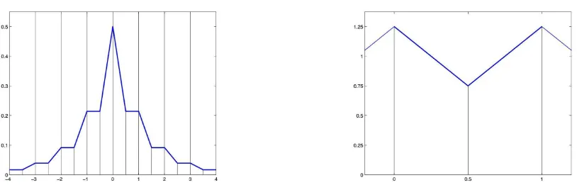
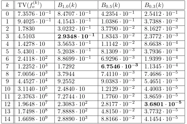
Then f is unimodal with mode at zero, whence TV(f) = 2f(0) = 2τ. Moreover, one verifies easily that g is linear and decreasing on [0,1/2] and linear and increasing on [1/2,1] with g(0)−g(1/2) =τ. Thus TV(g,[0,1]) = 2τ as well. Figure 1 illustrates this construction. The left panel shows (parts of) an even density f withf(0) = 0.5 = TV(f)/2, and the resulting functiong with TV(g,[0,1]) = TV(f) =g(1)−g(0.5).
As a corollary to Theorem 1 we obtain a refinement of the inequality
sup
0≤x≤1|
G(x)−x| ≤TV(f)/6
which was obtained by Pinkham (1961, corollary to Theorem 2) via Fourier techniques:
Corollary 2. Under the conditions of Theorem 1, for0≤x < y≤1,
¯
¯G(y)−G(x)−(y−x) ¯
¯ ≤ (y−x)(1−(y−x))TV(f)/2.
In particular,
Figure 1: A densityf (left) and the correspondingg (right) such that TV(f) = TV(g).
The previous results are for the case of TV(f) being finite. Next we consider smooth densities f. A function hon the real line is called k ≥1 times absolutely continuous if h∈ Ck−1(R),
and if its derivativeh(k−1) is absolutely continuous. Withh(k) we denote some version of the
derivative ofh(k−1)inL1 loc(R).
Theorem 3. Suppose thatf is k≥1 times absolutely continuous such that TV(f(k))<∞ for some version of f(k). Then g is Lipschitz-continuous on R. Precisely, for x, y
∈ R with |x−y| ≤1,
¯
¯g(x)−g(y) ¯
¯ ≤ |x−y|(1− |x−y|)
TV(f(k))
2·6k−1 ≤
TV(f(k))
8·6k−1 .
Corollary 4. Under the conditions of Theorem 3, for0≤x < y≤1,
¯
¯G(y)−G(x)−(y−x) ¯
¯ ≤ (y−x)(1−(y−x))
TV(f(k))
2·6k .
In particular,
KD(G) ≤ TV(f
(k))
8·6k and MRAE(G) ≤
TV(f(k))
2·6k .
Finally, let us note that Theorem 1 entails a short proof of the qualitative result mentioned in the introduction:
Corollary 5. LetY =µ+σYofor someµ∈R,σ >0and a random variableYowith density
fo, i.e. f(x) =fo((x−µ)/σ)/σ. Then
Z 1
0 |
g(x)−1|dx → 0 as σ→ ∞, uniformly inµ.
3
Some applications
We start with a general remark on location-scale families. Letfobe a probability density on
the real line such that TV(fo(k))<∞for some integerk≥0. Forµ∈Randσ >0 let
f(x) =fµ,σ(x) := σ−1f¡σ−1(x−µ)¢.
Then one verifies easily that
3.1
Normal and log-normal distributions
Forφ(x) := (2π)−1/2exp(−x2/2), elementary calculations reveal that
TV(φ) = 2φ(0) ≈ 0.7979, TV(φ(1)) = 4φ(1) ≈ 0.9679,
TV(φ(2)) = 8φ(√3) + 2φ(0) ≈ 1.5100.
In general,
φ(k)(x) = Hk(x)φ(x)
with the Hermite type polynomial
Hk(x) = exp(x2/2)
dk
dxk exp(−x
2/2)
of degreek. Via partial integration and induction one may show that
Z
Hj(x)Hk(x)φ(x)dx = 1{j=k}k!
for arbitrary integersj, k≥0 (cf. Abramowitz and Stegun 1964). Hence the Cauchy-Schwarz inequality entails that
TV(φ(k)) =
Z
|φ(k+1)(x)|dx
=
Z
|Hk+1(x)|φ(x)dx
≤ ³
Z
Hk+1(x)2φ(x)dx
´1/2
= p(k+ 1)!. These bounds yield the following results:
Theorem 6. Let f(x) = fµ,σ(x) = φ((x−µ)/σ)/σ for µ ∈ R and σ ≥ 1/6. Then the
corresponding functions g=gµ,σ andG=Gµ,σ satisfy the inequalities
R(gµ,σ) ≤ 4.5·h
¡
⌊36σ2
⌋¢
, KD(Gµ,σ) ≤ 0.75·h¡⌊36σ2⌋¢,
MRAE(Gµ,σ) ≤ 3·h
¡
⌊36σ2
⌋¢
,
where h(m) :=p
m!/mmfor integersm≥1.
It follows from Stirling’s formula thath(m) =cmm1/4e−m/2 with limm→∞cm= (2π)1/4. In
particular,
lim
m→∞
logh(m)
m = −
1 2,
so the bounds in Theorem 6 decrease exponentially in σ2. For σ = 1 we obtain already the
remarkable bounds
R(g) ≤ 4.5·h(36) ≈ 2.661·10−7,
KD(G) ≤ 0.75·h(36) ≈ 4.435·10−8,
MRAE(G) ≤ 3·h(36) ≈ 1.774·10−7
Corollary 7. For an integer baseb≥2 letX =bY for some random variableY
∼ N(µ, σ2)
with σ≥1/6. Then the leading digitsD0, D1, D2, . . . ofX satisfy the following inequalities:
For arbitrary digitsd0, d1, d2, . . .∈ {0,1, . . . , b−1}withd0≥1 and integersℓ≥0,
¯ ¯ ¯ ¯ ¯
P¡(Di)ℓi=0= (di)ℓi=0¢ logb(1 +b−ℓ/d(ℓ)) −
1
¯ ¯ ¯ ¯ ¯
≤ 3·h¡
⌊36σ2⌋¢
,
whered(ℓ):=Pℓ
i=1di·b−i. ¤
3.2
Gumbel and Weibull distributions
LetX >0 be a random variable with Weibull distribution, i.e. for some parametersγ, τ >0,
P(X ≤r) = 1−exp(−(r/γ)τ) forr≥0.
Then the standardized random variableYo:=τlog(X/γ) satisfies
Fo(y) := P(Yo≤y) = 1−exp(−ey) fory∈R
and has density function
fo(y) = eyexp(−ey),
i.e.−Yo has a Gumbel distribution. ThusY := logb(X) may be written asY =µ+σYo with
µ:= logb(γ) andσ= (τlogb)−1.
Elementary calculations reveal that for any integern≥1,
fo(n−1)(y) = pn(ey) exp(−ey)
withpn(t) being a polynomial intof degreen. Precisely,p1(t) =t, and
pn+1(t) = t(p′n(t)−pn(t)) (4)
forn= 1,2,3, . . .. In particular,p2(t) =t(1−t) andp3(t) =t(1−3t+t2). These considerations
lead already to the following conclusion:
Corollary 8. LetX >0 have Weibull distribution with parametersγ, τ >0 as above. Then TV(fo(k))<∞and
¯ ¯ ¯ ¯ ¯
P¡
(Di)ℓi=0= (di)ℓi=0
¢
logb(1 +b−ℓ/d(ℓ)) −
1
¯ ¯ ¯ ¯ ¯
≤ 3·TV(fo(k))
³τlogb
6
´k+1
for arbitrary integersk, ℓ≥0and digitsd0, d1, d2. . . as in Corollary 7. ¤
Explicit inequalities as in the gaussian case seem to be out of reach. Nevertheless some numerical bounds can be obtained. Table 1 contains numerical approximations for TV(fo(k))
and the resulting upper bounds
Bτ(k) := 3·TV(fo(k))
³τ log(10)
6
´k+1
k TV(fo(k)) B1.0(k) B0.5(k) B0.3(k)
0 7.3576·10−1 8.4707
·10−1 4.2354
·10−1 2.5412
·10−1
1 9.4025·10−1 4.1543·10−1 1.0386·10−1 3.7388·10−2
2 1.7830 3.0232·10−1 3.7790
·10−2 8.1627
·10−3
3 4.5103 2.9348·10−1
1.8343·10−2 2.3772
·10−3
4 1.4278·10 3.5653·10−1 1.1142
·10−2 8.6638
·10−4
5 5.4301·10 5.2038·10−1 8.1309
·10−3 3.7936
·10−4
6 2.4118·102 8.8699·10−1 6.9296·10−3 1.9399·10−4 7 1.2252·103 1.7292 6.7546
·10−3
1.1345·10−4
8 7.0056·103 3.7944 7.4110·10−3 7.4686·10−5 9 4.4527·104 9.2552 9.0383
·10−3 5.4651
·10−5
10 3.1140·105 2.4840·10 1.2129·10−2 4.4003·10−5
11 2.3763·106 7.2744
·10 1.7760·10−2 3.8659
·10−5
12 1.9648·107 2.3083·102 2.8177·10−2 3.6801·10−5
13 1.7498·108 7.8888
·102 4.8150
·10−2 3.7732
·10−5
14 1.6698·109 2.8890·103 8.8166·10−2 4.1454·10−5
Table 1: Some bounds for Weibull-distributedX withτ≤1.0,0.5,0.3
Remark. Writing
pn(t) = n
X
k=1
(−1)k−1Sn,k tk,
it follows from the recursion (4) that the coefficients can be calculated inductively by
S1,1 = 1, Sn,k=Sn−1,k−1+kSn−1,k.
Hence theSn,k are Stirling numbers of the second kind (see [6], chapter 6.1).
4
Proofs
4.1
Some useful facts about total variation
In our proofs we shall utilize the some basic properties of total variation of functionsh:J→R (cf. Royden 1988, Chapter 5). Note first that
TV(h,J) = TV+(h,J) + TV−(h,J)
with
TV±(h,J) := supn
m
X
i=1
¡
h(ti)−h(ti−1)¢
±
: m∈N;t0<· · ·< tm;t0, . . . , tm∈Jo
anda± := max(±a,0) for real numbersa. Here are further useful facts in case ofJ=R:
Lemma 9. Let h : R → R with TV(h) < ∞. Then both limits h(±∞) := limx→±∞h(x) exist. Moreover, for arbitrary x∈R,
In particular, ifh(±∞) = 0, thenTV+(h) = TV−(h) = TV(h)/2. ¤
Lemma 10. Lethbe integrable overR.
(a) IfTV(h)<∞, thenlim|x|→∞h(x) = 0.
While Lemma 9 is standard, we provide a proof of Lemma 10:
Proof of Lemma 10. Part (a) follows directly from Lemma 9. Since TV(h) <∞, there exist both limits limx→±∞h(x). If one of these limits was nonzero, the function hcould not be integrable overR.
For the proof of part (b), defineh(k)(±∞) := lim
4.2
Proofs of the main results
In particular, for two pointsx, y∈[0,1] with min(g(x), g(y))<∞, the difference g(x)−g(y) is finite. Hence g < ∞ everywhere. Now it follows directly from (5) that TV(g) ≤TV(f). Moreover, for 0≤x < y≤1,
where the latter equality follows from Lemma 10 (a) and Lemma 9. ¤
Proof of Corollary 2. Let 0≤x < y≤1 andδ:=y−x∈(0,1]. Then
Recall that lim|z|→∞f(j)(z) = 0 for 0 ≤ j ≤ k by virtue of Lemma 10 (b). In particular,
satisfies the inequality¯¯ ¯g Moreover, it follows from (6) that
¯
and, via dominated convergence,
lim
Now we perform an induction step: Suppose that for some 1≤j < k,
¯
These considerations show thatg(0)(x, y) := lim
N→∞gN(0)(x, y) always exists and satisfies the
In particular, g is everywhere finite with g(y)−g(x) = g(0)(x, y) satisfying the asserted
Proof of Corollary 4. For 0≤x < y≤1 andδ:=y−x∈(0,1],
Proof of Corollary 5. It is wellknown that integrable functions on the real line may be approximated arbitrarily well inL1(R) by regular functions, for instance, functions with
com-pact support and continuous derivative. With little extra effort one can show that for any fixedǫ >0 there exists a probability density ˜fo such that TV( ˜fo)<∞and
by means of Theorem 1. Sinceǫ >0 is arbitrarily small, this yields the asserted result. ¤
Proof of Theorem 6. According to Theorem 1,
R(gµ,σ) ≤
whereas Theorem 3 and the considerations in Section 3.1 yield the inequalities
for all k≥1. Since the right hand side equals 0.75/σ≥φ(0)/σ if we plug ink= 0, we may conclude that
R(gµ,σ) ≤
p
(k+ 1)!
8·6k−1σk+1 = 4.5·
s
(k+ 1)! (36σ2)k+1
for allk≥0. The latter bound becomes minimal ifk+ 1 =⌊36σ2
⌋ ≥1, and this value yields the desired bound 4.5·h¡
⌊36σ2
⌋¢
.
Similarly, Corollaries 2 and 4 yield the inequalities
KD(Gµ,σ) ≤
p
(k+ 1)!
8·6kσk+1 = 0.75·
s
(k+ 1)! (36σ2)k+1,
MRAE(Gµ,σ) ≤
p
(k+ 1)! 2·6kσk+1 = 3·
s
(k+ 1)! (36σ2)k+1,
for arbitraryk≥0, andk+ 1 =⌊36σ2⌋ ≥1 leads to the desired bounds. ¤
Acknowledgement. We are grateful to Steven J. Miller and an anonymous referee for con-structive comments on previous versions of this manuscript.
References
[1] M. AbramowitzandI.A. Stegun(1964). Handbook of Mathematical Functions with Formulas, Graphs, and Mathematical Tables. Dover, New York.
[2] F. Benford(1938). The law of anomalous numbers.Proc. Amer. Phil. Soc.78, 551-572.
[3] P. Diaconis(1977). The Distribution of Leading Digits and Uniform Distribution Mod 1. Ann. of Prob.5, 72-81. MR0422186
[4] R.L. Duncan(1969). A note on the initial digit problem. Fibonacci Quart.7, 474-475. MR0240036
[5] H.A. Engel,C. Leuenberger(2003). Benford’s law for exponential random variables. Stat. Prob. Letters63, 361-365. MR1996184
[6] R.L. Graham, D.E. Knuth, O. Patashnik(1994). Concrete Mathematics. A Foun-dation for Computer Science (2nd Edition). Addison-Wesley, Reading MA. MR1397498
[7] T.P. Hill(1995). A Statistical Derivation of the Significant-Digit Law.Statistical Science
10, 354-363. MR1421567
[8] T.P. Hill(1998). The First Digit Phenomenon. American Scientist86, 358-363.
[9] T.P. Hill,K. Schuerger(2005). Regularity of Digits and Significant Digits of Random Variables. Stochastic Proc. Appl.115, 1723-1743. MR2165341
[11] A.V. Kontorovich, S.J. Miller(2005). Benford’s law, values of L-functions and the 3x+ 1 problem. Acta Arithmetica120, 269-297. MR2188844
[12] D.E. Knuth(1981). The art of computer programming, Volume 2: seminumerical algo-rithms. Addison-Wesley, Reading MA. MR0633878
[13] L.M. Leemis,B.W. Schmeiser,D.L. Evans(2000). Survival Distributions Satisfying Benford’s Law. Amer. Statistician54, 1-6. MR1803620
[14] S.J. MillerandM.J. Nigrini(2006, revised 2007). Order statistics and shifted almost Benford behavior. Preprint (arXiv:math/0601344v2).
[15] S.J. MillerandM.J. Nigrini(2007). Benford’s Law applied to hydrology data - results and relevance to other geophysical data. Mathematical Geology39, 469-490.
[16] S. Newcomb (1881). Note on the frequency of use of the different digits in natural numbers. Amer. J. Math. 4, 39-40. MR1505286
[17] M. Nigrini (1996). A Taxpayer Compliance Application of Benford’s Law. J. Amer. Taxation Assoc.18, 72-91.
[18] R.S. Pinkham(1961). On the distribution of first significant digits. Ann. Math. Statist. 32, 1223-1230. MR0131303
[19] R. Raimi (1976). The First Digit Problem. Amer. Math. Monthly 102, 322-327. MR0410850