Full Terms & Conditions of access and use can be found at
http://www.tandfonline.com/action/journalInformation?journalCode=ubes20
Download by: [Universitas Maritim Raja Ali Haji] Date: 11 January 2016, At: 22:45
Journal of Business & Economic Statistics
ISSN: 0735-0015 (Print) 1537-2707 (Online) Journal homepage: http://www.tandfonline.com/loi/ubes20
The Trace Restriction: An Alternative Identification
Strategy for the Bayesian Multinomial Probit
Model
Lane F. Burgette & Erik V. Nordheim
To cite this article: Lane F. Burgette & Erik V. Nordheim (2012) The Trace Restriction: An Alternative Identification Strategy for the Bayesian Multinomial Probit Model, Journal of Business & Economic Statistics, 30:3, 404-410, DOI: 10.1080/07350015.2012.680416 To link to this article: http://dx.doi.org/10.1080/07350015.2012.680416
Accepted author version posted online: 03 Apr 2012.
Submit your article to this journal
Article views: 245
The Trace Restriction: An Alternative
Identification Strategy for the Bayesian
Multinomial Probit Model
Lane F. BURGETTE
RAND Corporation, Arlington, VA 22202 ([email protected])
Erik V. NORDHEIM
Department of Statistics, University of Wisconsin Madison, WI 53706 ([email protected])
Previous authors have made Bayesian multinomial probit models identifiable by fixing a parameter on the main diagonal of the covariance matrix. The choice of which element one fixes can influence posterior predictions. Thus, we propose restricting the trace of the covariance matrix, which we achieve without computational penalty. This permits a prior that is symmetric to permutations of the nonbase outcome categories. We find in real and simulated consumer choice datasets that the trace-restricted model is less prone to making extreme predictions. Further, the trace restriction can provide stronger identification, yielding marginal posterior distributions that are more easily interpreted.
KEY WORDS: Gibbs sampler; Marginal data augmentation; Prior distribution.
1. INTRODUCTION
In recent years, advances in Bayesian computation have made the multinomial probit (MNP) model an accessible and flexible choice for modeling discrete-choice data (e.g., Albert and Chib
1993; McCulloch and Rossi1994; Imai and van Dyk2005a,b). A central difficulty in the Bayesian computation of such mod-els has been the fact that the model is not identifiable unless a restriction is made on the covariance matrix (e.g., Train
2003, chap. 5). This restriction is necessary because we only observe the index of the maximum of the latent utilities that define the model; multiplying each utility by a positive constant preserves the ordering. The standard solution has been to require that the (1,1) element ofbe fixed at unity (e.g., Imai and van Dyk2005a; hereafter IVD). However, we find that the choice of which category corresponds to the unit variance element can have a large effect on the posterior predicted choice probabil-ities. (This is in contrast to maximum likelihood estimates of multinomial logit models, which are insensitive to the ordering of the outcomes.) An alternative identifying restriction—the one explored here—is to fix the trace of the covariance matrix, which obviates the choice of which single element to fix. Specifically, we discuss adapting the Gibbs sampler of Imai and van Dyk (2005a) to accommodate the trace restriction. We achieve this without any computational penalty relative to the IVD sampler. We will make three main arguments for the use of the trace restriction over the standard approach. The first appeals to sym-metry: Using the trace restriction allows us to specify a prior for
that is invariant to joint permutations of its rows and columns. We argue that this is a desirable feature of an objective prior for the MNP model. On the other hand, we will show in a special case that a standard IVD prior specification yields very different prior expectations for the diagonal elements of.
Second, in real and simulated datasets, we find that the trace-restricted fits tend to have behavior that is intermediate in the range of models that result from the IVD priors. That is to say, the
trace-restricted prior tends to provide posterior predictions that are between those resulting from IVD priors that use the various identifying assumptions. Thus, using the trace restriction seems to take some of the volatility out of the modeling process.
Third, we find that the trace restriction yields marginal poste-rior distributions that can be easier to interpret. As an example of this, we present an analysis where identification essentially breaks down when using a standard IVD restriction. This gives the impression that the regression coefficients’ marginal poste-rior distributions are strongly bimodal when a stronger identifi-cation strategy would not indicate such behavior. We find that the trace restriction is less susceptible to this difficulty.
In this article, we consider only the issue of setting the scale of the latent utilities. However, a similar sensitivity to the spec-ification of the base category can be a problem. We reserve this issue for future research.
The remainder of the article is arranged as follows. In the next section, we review the Gibbs sampler of Imai and van Dyk (2005a). In Section3, we motivate and derive the new trace-restricted Gibbs sampler. Section4 presents an application of our methods to a real example, along with a simulation study based on the real-data analysis. In Section5, we provide some discussion of our method, and we conclude with Section6.
2. THE BAYESIAN MNP MODEL OF IMAI AND VAN DYK (2005)
The MNP model is a flexible tool for modeling discrete choices. MNP models do not specify a rigid covariance struc-ture as multinomial logit models typically do. Standard multi-nomial logit models make the assumption of independence of
© 2012American Statistical Association Journal of Business & Economic Statistics July 2012, Vol. 30, No. 3 DOI:10.1080/07350015.2012.680416
404
Burgette and Nordheim: Trace Restriction for Multinomial Probit Model 405
irrelevant alternatives (IIA). This assumption means that the ratio of the probabilities of selection for two of the alterna-tives does not depend on the characteristics of other alternaalterna-tives (McFadden,1974; Train,2003, sec. 3.3.2). MNP models do not make the IIA assumption. However, we will see that the cost of the MNP’s flexibility is computational difficulty. Whereas logit models have closed forms for the likelihood, calculating MNP probabilities directly requires a computationally demanding integration.
We can define the MNP model through Gaussian latent vari-ables. We assume that decision maker (or agent)i=1, . . . , nis choosing amongp+1 mutually exclusive alternatives. Since the mean level of the utilities is not an identifiable quan-tity, we work with p-dimensional vectors of utilities. We as-sume that each agent forms a vector of latent utilities Wi =
(wi1, . . . , wip)′ with a dimension for each of the alternatives,
relative to a base alternative. The decision maker then chooses the option with the largest utility. Thus, the response variable is
Yi =
EachXican contain covariates that vary across agents (e.g.,
age) and/or those that vary among the (p+1) alternatives (e.g., product prices). In the models presented in this article, we work with prices and intercepts, so each Xi =[Ip,di], where Ip is
the identity matrix and di is a p-vector of differences in log prices between each alternative and the base alternative. Agent-specific covariates could be added by concatenatingxiIptoXi,
wherexi is a scalar covariate related to agenti.
Evaluation of the likelihood requires integrating out theWi.
This difficulty is avoided by using the Bayesian approach ofdata augmentation, wherein the latentWi are treated like unknown
parameters (Tanner and Wong1987). In such algorithms, the parameter space is augmented with the latent Wi. Thus, in a
Gibbs sampler, the latent Wi are sampled rather than being
analytically integrated out (e.g., Robert and Casella2004, chaps. 9 and 10).
Albert and Chib (1993) first demonstrated that data augmen-tation is a powerful tool for MNP calculations. Since condition-ing on the latentW and the observed responseY is the same
as conditioning only on W, we can use this approach to
cir-cumvent the integration necessary to calculate the likelihood. Data augmentation algorithms alternate between making draws fromp(θ|W,Y) and p(W|θ,Y), whereθ denotes the model parameters.
Since multiplying both sides of (2) by a positive constant does not change the outcome Yi, Imai and van Dyk (2005a)
setσ11=1 to achieve identifiability, where= {σij}. In their
preferred “Scheme 1” (on which we focus), IVD used the prior distributions
whereνis the prior degrees of freedom (an integer greater than or equal to the number of columns in) andSis the prior scale
whose (1,1) element is set at unity. These priors are chosen because of their computational properties, as we shall discuss below.
2.1 Marginal Data Augmentation
IVD transformed (2) by multiplying both sides by a positive, scalar parameterα. Thus, they had
αWi≡W˜i =Xiβ˜+ε˜i, where ε˜i ∼N(0,˜), (4)
with ˜≡α2and ˜β
≡αβ. Parameters such asαthat are not identifiable, given the data, but are identifiable in the expanded parameter space of a data augmentation algorithm are called working parameters(Meng and van Dyk1997). A working pa-rameter is helpful here because the transformed ˜is symmetric and positive-definite, but otherwise unconstrained. If one speci-fies the prior distribution ˜∼inv-Wishart (ν,S), then the prior
of (α2=σ11,=(α2)−1˜) is
the analyst is free from relying on the Metropolis–Hastings steps that were required to samplein the original Albert and Chib (1993) MNP sampler. Draws of ˜—and by transformation (α2,)—can be made through draws from a standard inverse-Wishart distribution. Because the conjugate prior forβis also used, only standard draws are needed.
Second, the IVD model has a transparent prior distribu-tion compared with some other fully MNP Gibbs samplers. McCulloch and Rossi (1994) proposed a model that specifies a prior distribution on ( ˜β,˜) and then “post-processes” back to (β,) by dividing, for example, the sampled ˜β values by the sampled values of √σ˜11. But this implies a complicated,
nonstandard prior for β (Imai and van Dyk2005a, sec.4.1). Relatedly, it is not possible to specify the noninformative prior p(β)∝1 in the McCulloch and Rossi model, whereas setting
B0=0in the IVD model gives that prior.
Finally, IVD argued that by giving α2 a distribution with positive variance, they had improved the mixing of the Gibbs sampler. Any proper prior may be assigned to working param-eters without affecting the posterior distribution of the model parameters, but there may be differences in the characteris-tics of the Markov chain that results. In particular, IVD ar-gued that we expect
p(Y,W|θ, α)p(α|θ)dα to be more dif-diffuse—as can be achieved with working parameters. Van Dyk (2010) made these arguments in greater depth and provided examples to support the claims.
Algorithms that make use of distributions for the working parameters are calledmarginal data augmentationalgorithms,
in contrast toconditional data augmentation. Through compar-ative applications, IVD showed that their algorithm has better convergence properties than other approaches that do not make such effective use of marginal data augmentation. Especially compared with the MNP algorithm of McCulloch, Polson, and Rossi (2000), which is a conditional data augmentation algo-rithm, the IVD sampler has very favorable mixing properties.
3. THE TRACE-RESTRICTED MNP
3.1 Motivation
Although the IVD priors are of a standard form, the prior specification requires a choice that may not be transparent. In particular, the model requires us to specify one of the outcome categories to correspond to the fixed element in the covariance matrix. This choice can affect the fitted model, but it seems highly unlikely that a researcher could be able to say which of the possible restrictions best matches his or her prior beliefs.
As an example, consider the IVD prior when is 2×2, S=I, andν=3; this serves as a default prior when there are three outcome categories in the software of Imai and van Dyk (2005b). In this simple case, we have closed forms for the prior of the free parametersσ22 andσ12. In particular, we have the
marginal prior
p(σ22)∝√σ22(1+σ22)−3. (6)
One can then show that the prior median ofσ22is 1, butE(σ22)=
3. Since E(σ11)=1, the choice of which outcome category
corresponds to the leading element ofcan impact inference. We will demonstrate later in the article that these differences can lead to meaningful differences in the posterior distribution. Using the trace restriction, on the other hand, we are able to definep() that is invariant to permutations of the subscripts of
= {σij}. This symmetry is a desirable property of an objective
Bayesian prior.
3.2 A Trace-Restricted MNP Gibbs Sampler
To implement the trace-restricted MNP, we follow the spirit of the IVD model structure. We start with a ˜that is symmetric and positive-definite, but otherwise unrestricted. We then transform
˜
to (α2,), whereα2=tr( ˜)/pand=˜/α2. We assume that ˜ has an inverse-Wishart distribution with parameters ν and S and tr(S)=p. The Jacobian of this transformation is
proportional toαp(p+1)−2, and therefore is proportional to the Jacobian of the IVD calculation. (This derivation relies on the identity det(In+U′V)=det(Im+V U′) form×n matrices
UandV (see corollary 18.1.2 of Harville (2008)).
Making the transformation, it follows that
p(α2,)∝ ||−(ν+p+1)/2
exp{−tr(α−2S−1
)/2}(α2)−(pν+2)/2, (7)
whereis restricted so that it is symmetric and positive-definite and satisfies tr()=p. This is exactly the same asp(α2,) for
IVD, except there is a different constraint on. Therefore, p()∝ ||−(ν+p+1)/2[tr(S−1)]−pν/21{tr()=p}. (8)
It is convenient that the IVD and trace-restricted priors are so similar. Because p(α2,) is the same for both algorithms
(except for the restriction on), draws conditioning onare the same in each scheme. Also, the two methods have the same prior p( ˜). Hence, the only computational difference is the transformation from ˜to (α2,).
Therefore, following IVD, the steps of the trace-restricted MNP Gibbs sampler are
(1) Draw wij and α2 jointly, given β, , Y, and the other
components ofW (wij andαare independent given).
• For eachiand 1≤j ≤p, samplewij, given the other
components ofWi,β, and. This requires a draw from a truncated univariate normal distribution.
• Then draw from p(α2
|β,,Y)=p(α2
|). This dis-tribution is a scaled inverse chi-square: (α2
|)∼
To emphasize, only the second part of Step (3) differs from the IVD algorithm (in the IVD algorithm, we setα2
=σ˜11).
4. APPLICATIONS
4.1 Margarine Purchases
We consider records of margarine purchases that were recorded in the ERIM database, which was collected by A.C. Neilsen in the mid-1980s (McCulloch and Rossi1994) (see also
http://research.chicagobooth.edu/marketing/databases/erim). Like McCulloch and Rossi, we limit ourselves to families that purchased at least one of Parkay, Blue Bonnet, Fleischmann’s, house brand, generic, or Shedd Spread Tub margarines and model the purchase probabilities as a function of (log) prices. Further, for simplicity, we only consider the first recorded purchase of one of these brands for each household, which results in 507 observations. The margarine data are available in thebayesmpackage in R.
We fit these data using a single-base category (Blue Bonnet brand) and the various identifying assumptions for. That is to
Burgette and Nordheim: Trace Restriction for Multinomial Probit Model 407
Figure 1. Estimated purchase probabilities of “House brand” mar-garine for a range of prices, with the other prices fixed at those from the first observation. The solid black line uses the trace restriction. The broken black line uses House brand as the fixed element in the covariance under the IVD identification strategy. Four overplotted gray lines represent the predictions when other brands correspond to fixed element in the covariance matrix.
say, we fit the model repeatedly, considering fits with each of the nonbase categories used to set the scale of the model, as well as using the trace restriction. In this example with a modest sample size, we find considerable discrepancies between the predictions that result from the various model fits. For all of these fits, we use a prior somewhat stronger than the MNP software defaults, with ν=8 instead of the defaultν=6 (Imai and van Dyk2005b) because of numerical instability when we do not use the trace restriction. We also use the noninformative priorp(β)∝1.
We consider plots of predicted purchase probabilities as price changes for a particular brand, with the other prices staying fixed. Such predictions could be useful for a brand manager when deciding on price changes or designing promotional of-fers, as they could be used to predict market share if the competi-tors’ prices stay fixed. InFigure 1, we use the prices associated with the first observation in our data and consider a range of alternative prices for the “House brand” stick margarine. Here, we observe that the purchase probabilities of the House brand tend to be less affected by price when House brand corresponds to the fixed variance component (broken line) compared with when another brand sets the scale (overplotted gray lines). On the other hand, the posterior selection probabilities associated with the trace-restricted fit (solid black line) fall somewhere between these.
If we fit the models with larger ν values, the differences in predictions diminish, but remain meaningfully large for a range of degrees of freedom. For instance, withν =10, the House brand selection probabilities still differ by more than 15% for various IVD restrictions at the low end of our price range. Forν=12, this difference is around 5%. Whenν≥15, the discrepancies are essentially gone.
Further, we note that the trace restriction proves to identify the model more strongly in this modest-sample-size application. If we fit the model usingν =6 degrees of freedom, uncertainty in the scale can cause the estimated parameters to effectively
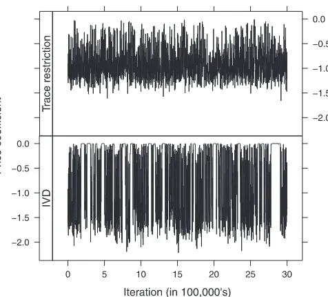
Figure 2. Thinned trace plots of price coefficients for trace-restricted and IVD identifying approaches from chains of length 3 million, using the margarine data andν=6 prior degrees of freedom. The flat-topped peaks indicate a collapse to zero for the IVD chain because of a weak identifying restriction.
collapse to zero, as observed from the flat-topped spikes in the trace plot for the price coefficient using an IVD prior (see
Figure 2). In such a case, the joint distribution of the estimated parameters (and the corresponding predictions) may contain meaningful information, but posterior marginal distributions may not be interpretable. For instance, consider the marginal posterior distribution of the price coefficient estimated using the IVD restriction, with Blue Bonnet as the fixed variance (see
Figure 3). The distribution is strongly bimodal, appearing to be a mixture of distributions centered at –1.5 and near zero. Comparing this to the trace-restricted fit (or to an IVD fit with a largerν), we observe that the bimodality is an artifact of a poor identifying restriction. Note that only the prior on (and not onβ) changes between these two fits.
We have also found that this collapse of identification can lead to numerical instability, with draws of that are nearly singular. In practice, the instability of these estimates can be
Figure 3. Density histogram of sampled price coefficients with trace-restricted and IVD priors for the margarine data. These are from the chains whose trace plots are displayed inFigure 2. The bimodality of the IVD fit is an artifact of a poor identifying restriction.
addressed with regularization through a more informative prior, as we did with the ν=8 fits reported in Figure 1. However, using a largerνto more strongly identify the scale will lead to a prior that is more informative about the correlation structure in, which may be undesirable. It is an appealing aspect of the trace-restricted MNP that it provides more stable estimates than other restrictions when using a small value ofν.
4.2 Simulated Data
We now apply MNP models to simulated data using the trace and single-element identifying restrictions. For each repetition of the simulation, we draw 500 sets of prices (with replacement) from the data used in the margarine analysis. We draw intercepts independently and uniformly from the interval [−0.25,0.25] and price coefficients from the interval [−1.5,−0.5]. These distributions correspond to plausible models in marketing ap-plications, and heavy-tailed distributions for these components would be more likely to produce datasets in which certain brands were not purchased, which we do not allow. We also draw an unnormalized covariance matrix from an inverse-Wishart distri-bution with 25 degrees of freedom that is centered at the identity matrix.
After simulating purchases, we then fit the data and compare differences between the true purchase probabilities and posterior estimated purchase probabilities under the various identifying restrictions on . We measure differences between true and estimated purchase probabilities via the total variation norm, which is defined to be
0.5
y
|PrT(Yi =y)−PrE(Yi =y)|, (9)
where PrT and PrE indicate the true and estimated purchase
probabilities, respectively, taking covariates into account (e.g., Johnson1998). In the sum,yindexes the available brands. We report these differences averaged across the first 50 sets of prices in each simulated dataset. We specifyν=8, which makes the prior stronger than the defaultν=6 and improves mixing of the Markov chains. This, along with the use of 500,000 post burn-in iterations, makes the Monte Carlo errors generally small.
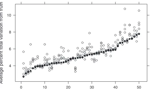
InFigure 4, we plot the average percent total variation dis-tance from the truth for each identifying restriction and each generated dataset. We observe that the trace restriction consis-tently performs well. In 17 out of 50 runs, it produces predic-tions that are closest to the truth. In only one of these runs (the repetition labeled 23) does it have the largest discrepancy from the truth. These results are consistent with the idea that the trace restriction tends to give predictions that are between those of the various IVD restrictions, in the sense ofFigure 1.
5. DISCUSSION
5.1 Convergence
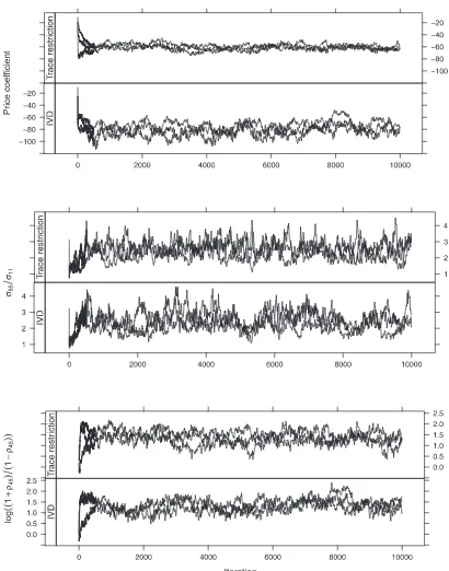
Since one of the main successes of the IVD algorithm is its mixing behavior, it is worth comparing the results of IVD with those of the trace-restricted sampler. Because the algorithms are so similar, it is not surprising that their mixing behaviors also seem to be very similar. InFigure 5, we display the terms
Figure 4. Percent total variation from true probabilities, averaged across the first 50 sets of prices in each of the 50 simulated datasets. Hollow circles are from IVD identifying restrictions, and solid circles are from the trace restriction. The repetitions are arranged based on the distance of the trace restriction’s estimates from the truth.
selected by IVD for their comparisons with the other Bayesian MNP methods in their analysis of consumers’ purchases of clothing detergent. The differences between the IVD algorithm and the other previous MNP samplers are striking in terms of the number of iterations required to reach convergence. Such obvious differences do not exist here. Perhaps, the price coeffi-cient for the trace-restricted fit is slightly slower in converging to the area of high posterior density, but such differences do not seem to be consistent across runs and models.
5.2 Comparison With the MNP Model of McCulloch and Rossi (1994)
An alternative approach to the MNP specifies a prior on ˜βand then post-processes to bring the estimates into an identifiable scale by dividing sampled ˜βj components by σ˜j
11, where j
indexes the iteration in the Markov chain (McCulloch and Rossi
1994; hereafter MR) (see also Rossi, Allenby, and McCulloch
2005). This post-processing is necessary if one is interested in summaries of the model parameters. The predictions, however, are insensitive to the choice of the category that sets the scale in the post-processing, or whether one post-processes at all. Thus, the MR and trace-restricted MNP models share the property that they are not sensitive to reordering the nonbase categories.
Although the MR algorithm is easy to implement and the re-sulting Markov chains have been found to have favorable mix-ing properties, the model does introduce two difficulties. First, the prior is specified on the unidentified regression parameters ( ˜β,˜). The prior that is induced on the identifiable parameters is nonstandard, and it may be harder for practitioners to match to prior beliefs. Second, as McCulloch and Rossi emphasized in a later work with Polson, “it is impossible to specify a truly diffuse or improper prior with [the MR] approach” (McCulloch, Polson, and Rossi2000, p. 174).
Lacking a “truly diffuse” prior, an analyst in the MR frame-work may think it reasonable to substitute a proper yet high variance prior for ˜β. To evaluate the merits of such an approach, we expand the simulation in Figure 4 (using identical simu-lated datasets) to include results from an MR model that uses a
Burgette and Nordheim: Trace Restriction for Multinomial Probit Model 409
Figure 5. Trace plots for parameters highlighted by IVD in their detergent analysis. For both algorithms, the Markov chains quickly converge to areas of high posterior density.
normal prior for ˜β centered at zero, with a standard devia-tion of 1000. Recall that p(β)∝1 for the models in
Fig-ure 4. We use the same ν=8 degrees of freedom for each model.
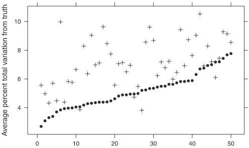
Figure 6summarizes the results, again measuring prediction error via the average percent total variation between true se-lection probabilities and the corresponding posterior estimates. The solid circles—from the trace-restricted model—are identi-cal to those inFigure 4. The plus signs are analogous quantities from the MR model output. We observe that the MR models with large prior variance usually do worse than trace-restricted
model, sometimes significantly so. Averaged across repetitions of the simulation, the MR error is around 7.1%, compared with 5.2% for the trace-restricted model.
To summarize the comparison of these models, the MR and trace-restricted models are similar in several key respects: They are computationally straightforward, the associated Gibbs al-gorithms mix relatively well, and the predictions are invari-ant to relabeling the nonbase outcome categories. However, the MR model specifies priors on β indirectly and does not allow us to specify a flat prior onβ. This simulation gives evi-dence that proper yet high variance priors for ˜βmay be a poor
Figure 6. Percent total variation from true probabilities, averaged across the first 50 sets of prices in each of the 50 simulated datasets. Circles are from the trace restriction, and plus signs are from the McCulloch and Rossi model. The repetitions are arranged based on the distance of the trace restriction’s estimates from the truth.
substitute—in terms of out-of-sample prediction—for the im-proper priors that are available in the IVD framework.
6. CONCLUSION
The IVD prior requires the analyst to make an arbitrary choice in specifying the constraint required for the procedure. In a real-data application, we found that the choice of which IVD restric-tion we use can have a large impact on features of the poste-rior distribution: Changes of around 20% for predicted purchase probabilities may lead a company to make very different pricing decisions. We instead suggest a prior that is invariant to rela-beling the rows and columns of the covariance matrix. We find that the trace restriction tends to provide “moderate” inference, insofar as predictions tend to be between those of the different possible IVD priors. In short, we find that the trace restriction yields better properties as an objective Bayesian prior.
Sensitivity to the identifying restriction is the result of influ-ence of the prior. Therefore, if a sufficient amount of data has accrued, we do not expect differences based on which identify-ing restriction one uses. For example, usidentify-ing the detergent data that IVD discussed, posterior predictions appear identical under the various restrictions. This dataset has around five times as many observations for the same number of parameters as the margarine data used in this article, so the prior plays a much weaker role in the analysis of the detergent data.
More broadly, the need to constrain certain quantities in Bayesian models to achieve identification is not unique to the MNP. This research suggests that it may be advantageous in other models to work with identifying restrictions that are
symmetric with respect to the group of parameters that are being restricted. As an example of this, a referee noted that Strachan and Van Dijk (2008) took this general approach, requiring that
ββ′=Irather than placing restrictions on individual elements,
whereβis a matrix of coefficients in the vector error correction model. We hope that such symmetric restrictions will become more widely used in Bayesian modeling.
ACKNOWLEDGMENTS
The authors thank the editor Keisuke Hirano, an associate editor, and two anonymous referees for suggestions that signifi-cantly improved the manuscript. The authors also thank Kosuke Imai for his thoughtful comments and for adding the trace re-striction to the MNP package.
[Received December 2009. Revised February 2012.]
REFERENCES
Albert, J., and Chib, S. (1993), “Bayesian Analysis of Binary and Polychoto-mous Response Data,” Journal of the American Statistical Association, 88(422), 669–679. [404,405]
Harville, D. (2008),Matrix Algebra From a Statistician’s Perspective, New York: Springer-Verlag. [406]
Imai, K., and van Dyk, D. (2005a), “A Bayesian Analysis of the Multinomial Probit Model Using Marginal Data Augmentation,”Journal of Economet-rics, 124(2), 311–334. [404,405]
——— (2005b), “MNP: R Package for Fitting the Multinomial Probit Model,”
Journal of Statistical Software, 14(3), 1–32. [404,406]
Johnson, V. (1998), “A Coupling-Regeneration Scheme for Diagnosing Conver-gence in Markov Chain Monte Carlo Algorithms,”Journal of the American Statistical Association, 93(441), 238–248. [408]
McCulloch, R., Polson, N., and Rossi, P. (2000), “A Bayesian Analysis of the Multinomial Probit Model With Fully Identified Parameters,”Journal of Econometrics, 99(1), 173–193. [406,408]
McCulloch, R., and Rossi, P. (1994), “An Exact Likelihood Analysis of the Multinomial Probit Model,”Journal of Econometrics, 64(1), 207–240. [404,405,406]
McFadden, D. (1974), “The Measurement of Urban Travel Demand,”Journal of Public Economics, 3(4), 303–328. [405]
Meng, X., and van Dyk, D. (1997), “The EM Algorithm—an Old Folk-Song Sung to a Fast New Tune,”Journal of the Royal Statistical Society,Series B Methodologicals, 511–567. [405]
Robert, C., and Casella, G. (2004),Monte Carlo Statistical Methods, New York: Springer-Verlag. [405]
Rossi, P., Allenby, G., and McCulloch, R. (2005),Bayesian Statistics and Mar-keting, Chichester: Wiley. [408]
Strachan, R., and Van Dijk, H. (2008), “Bayesian Averaging Over Many Dy-namic Model Structures With Evidence on the Great Ratios and Liquidity Trap Risk,” Technical Report 08-096/4, Tinbergen Institute, Rotterdam The Netherlands. [410]
Tanner, M., and Wong, W. (1987), “The Calculation of Posterior Distributions by Data Augmentation,”Journal of the American Statistical Association, 82(398), 528–540. [405]
Train, K. (2003), Discrete Choice Methods With Simulation, Cambridge: Cambridge University Press. [404]
van Dyk, D. A. (2010), “Marginal Markov Chain Monte Carlo Methods,” Sta-tistica Sinica, 20(4), 1423–1454. [405]