Full Terms & Conditions of access and use can be found at
http://www.tandfonline.com/action/journalInformation?journalCode=ubes20
Download by: [Universitas Maritim Raja Ali Haji] Date: 12 January 2016, At: 23:12
Journal of Business & Economic Statistics
ISSN: 0735-0015 (Print) 1537-2707 (Online) Journal homepage: http://www.tandfonline.com/loi/ubes20
Multivariate Tests of Mean–Variance Efficiency
With Possibly Non-Gaussian Errors
Marie-Claude Beaulieu, Jean-Marie Dufour & Lynda Khalaf
To cite this article: Marie-Claude Beaulieu, Jean-Marie Dufour & Lynda Khalaf (2007)
Multivariate Tests of Mean–Variance Efficiency With Possibly Non-Gaussian Errors, Journal of Business & Economic Statistics, 25:4, 398-410, DOI: 10.1198/073500106000000468
To link to this article: http://dx.doi.org/10.1198/073500106000000468
Published online: 01 Jan 2012.
Submit your article to this journal
Article views: 72
View related articles
Multivariate Tests of Mean–Variance Efficiency
With Possibly Non-Gaussian Errors: An Exact
Simulation-Based Approach
Marie-Claude B
EAULIEUCIRANO and Department of Finance and Insurance, Laval University, Ste-Foy, Quebec, Canada G1K 7P4 (Marie-Claude.Beaulieu@fas.ulaval.ca)
Jean-Marie D
UFOURCIRPEE, CIREQ, and Department of Economic Science, University of Montreal, Montreal, Quebec, Canada H3C 3J7 (jean.marie.dufour@umontreal.ca)
Lynda K
HALAFCIREQ, GREEN, and Department of Economics, Carleton University, Ottawa, Ontario, Canada K1S 5B6 (lynda-khalaf@carleton.ca)
We develop exact mean–variance efficiency tests of the market portfolio in the context of (conditional and unconditional) capital asset pricing models (CAPM), allowing for a wide class of possibly non-Gaussian error distributions. The proposed procedures are applicable in a general multivariate linear regression framework, and exactness is achieved through Monte Carlo test techniques. We also perform exact multi-variate diagnostic checks. Empirical results show that the Gaussian assumption is rejected, temporal insta-bilities are apparent, and mean–variance efficiency is rejected over several subperiods, but finite-sample methods that allow for nonnormality and conditioning information substantially reduce the number of rejections.
KEY WORDS: Bootstrap; Capital asset pricing model; Generalized autoregressive conditional het-eroscedasticity; Monte Carlo test; Multivariate linear regression; Nonnormality.
1. INTRODUCTION
The capital asset pricing model (CAPM) is one of the most commonly used models in theoretical and applied finance; (for reviews and references, see Campbell, Lo, and MacKin-lay 1997; Shanken 1996; Cochrane 2001; DeRoon and Nij-man 2001; Fama and French 2004). Since the work of Gibbons (1982), empirical tests on the CAPM are often conducted within amultivariate linear regression (MLR). In this context, stan-dard asymptotic theory provides a poor approximation to the finite-sample distribution of test statistics, even with fairly large samples (see Shanken 1996, sec. 3.4.2; Campbell et al. 1997, chap. 5; Dufour and Khalaf 2002b). In particular, test size dis-tortions grow quickly when the number of equations increases. As a result, the conclusions of MLR-based empirical studies on the CAPM can be strongly affected and can lead to spurious rejections.
Consequently, several exact and Bayesian methods have been proposed to assess mean–variance efficiency (see Job-son and Korkie 1982; MacKinlay 1987, 1995; Gibbons, Ross, and Shanken 1989 [henceforth GRS]; Stewart 1997; Kandel, McCulloch, and Stambaugh 1995). These methods typically require Gaussian distributional assumptions. However, it has long been recognized that financial returns exhibit nonnormal-ities (Fama 1965). Although the CAPM can be derived from expected utility maximization under various non-Gaussian as-sumptions on the return cross-sectional distribution, such as the multivariate t (see Ingersoll 1987; Berk 1997), finite-sample tests for mean–variance efficiency in non-Gaussian CAPMs are not yet available.
Indeed, mean–variance efficiency tests that relax normal-ity include (a) large-sample GMM or bootstrap techniques (Affleck-Graves and McDonald 1989; MacKinlay and Richard-son 1991; Fama and French 1993; Jagannathan and Wang 1996; Ferson and Harvey 1999; Groenwold and Fraser 2001); (b) semiparametric asymptotic procedures specific to ellipti-cal distributions (Hodgson, Linton, and Vorkink 2002; Vorkink 2003; Hodgson and Vorkink 2003); (c) parametric procedures based on postulating a non-Gaussian distribution, such as the multivariatet (Fiorentini, Sentana, and Calzolari 2003; Zhou 1993); and (d) non-Gaussian Bayesian procedures (Tu and Zhou 2004). In all of these approaches, the distributional the-ory of test statistics is either approximate or does not formally take into account nuisance parameter uncertainty in a fitted parametric distribution. In particular, Hodgson et al. (2002) reported size problems on high-dimensional systems and re-stricted their analysis to systems with three or four portfolios, whereas Vorkink (2003) proceeded on a portfolio-by-portfolio basis, not on the whole system. In the parametric case, Zhou (1993) proposed simulation-basedpvalues for the GRS statis-tic given a few ellipstatis-tical distributions, while selecting their tail area parameters by trial and error.
In this article we propose finite-sample unconditional and conditional multivariate mean–variance efficiency tests in pos-sibly non-Gaussian CAPMs. The conditional specifications allow model coefficients to vary as functions of a number
© 2007 American Statistical Association Journal of Business & Economic Statistics October 2007, Vol. 25, No. 4 DOI 10.1198/073500106000000468
398
of instruments, as described by Shanken (1996, sec. 2.3.4), Cochrane (2001, chap. 8), and DeRoon and Nijman (2001). Conditional testing is important because portfolios that are conditionally efficient might be unconditionally inefficient (see Hansen and Richard 1987; Cochrane 2001, chap. 8).
We use finite-sample results from Dufour and Khalaf (2002b) on testinguniform linear(UL) restrictions in MLR models with a given, possibly non-Gaussian, disturbance distribution. For such hypotheses, the null distributions of standard test statis-tics are invariant to MLR coefficients and error variances and covariances. In this case, Monte Carlo (MC) test techniques (see Dufour 2006) can be applied to obtain exact p values. On observing that mean–variance efficiency restrictions take the UL form when the risk-free rate is observable, we show that efficiency can be tested exactly under general distribu-tional assumptions that include the Gaussian and a wide spec-trum of non-Gaussian distributions, both elliptically symmetric and nonelliptical. Single- and multi-beta models are covered by these results.
To control for the parameters that define the hypothesized non-Gaussian distribution, such as the degrees of freedom for the multivariatet(a problem not considered in Dufour and Kha-laf 2002b), we use a two-stage procedure as follows: (1) We build an exact confidence set (with level 1−α1) for the nuisance parameter, through “inversion” of a distributional goodness-of-fit (GF) test, and (2) maximize the p value for the mean– variance efficiency test (which depends on the nuisance para-meter) over this confidence set. Referring the lattermaximized MC (MMC) p value to anα2 cutoff provides a test with ex-act levelα1+α2 (see Dufour and Kiviet 1996; Dufour 2006). We stick here to the original notion of test level in the presence of nuisance parameters (Lehmann 1986, chap. 3): A test has
levelαif the probability of rejecting the null hypothesis is not greater thanαfor any data-generating process compatible with the null hypothesis.
Furthermore, we evaluate the specification of the model us-ing GF tests on the error distribution and serial dependence tests. All procedures rely on properly standardized multivari-ate ordinary least squares (OLS) residuals, which provide sta-tistics invariant to MLR coefficients and error variances and covariances and allows easy application of MC tests. The GF tests compare multivariate skewness and kurtosis criteria with a simulation-based estimate of their expected value un-der the hypothesized (normal or nonnormal) distribution, which can be viewed as extensions of Mardia’s (1970) procedures. The diagnostic checks combine (as in Shanken 1990) stan-dardized individual-equation versions of the generalized au-toregressive conditional heteroscedasticity (GARCH) tests sug-gested by Engle (1982) and Lee and King (1993), and the variance-ratio tests of Lo and MacKinlay (1988); we also test for heteroscedasticity linked to conditioning on market returns (Vorkink 2003). Our exact combination method relies on sim-ulation (as in Dufour and Khalaf 2002a and Dufour, Khalaf, Bernard, and Genest 2004) to avoid the Bonferroni bounds ap-plied by Shanken (1990). Such bounds require one to divide the level of each individual test by the number of tests, lead-ing to possibly large power losses if the MLR includes many equations (i.e., many portfolios). All tests are performed under normal and nonnormal error distributions.
The proposed tests are applied to an unconditional and a con-ditional CAPM with observable risk-free rates and both mul-tivariate normal and mulmul-tivariate t distributions. We consider monthly returns on New York Stock Exchange (NYSE) portfo-lios, constructed from the University of Chicago Center for Re-search in Security Prices (CRSP) database (1926–1995). Our results show the following: (a) Multivariate normality is re-jected; (b) multivariate residual checks suggest temporal insta-bilities for both the unconditional and the conditional models; (c) although mean–variance efficiency is rejected over several subperiods, using finite-sample methods and allowing for non-normal errors reduces the number of subperiods for which effi-ciency is rejected and the strength of the evidence against it; and (d) using conditioning information has nonnegligible effects on tests of mean–variance efficiency and substantially reduces the number of rejections.
The article is organized as follows. In Section 2 we set up the framework. In Section 3 we describe existing tests and propose extensions for nonnormal distributions. In Section 4 we discuss how to deal with nuisance parameters in the error distribution. We describe GF and diagnostic tests in Section 5 and report the empirical results in Section 6. We conclude in Section 7.
2. FRAMEWORK
Let Rit, i=1, . . . ,n, be returns on n securities for
pe-riod t, and let R˜Mt be the return on a benchmark portfolio
(t=1, . . . ,T). Following Gibbons et al. (1989), the (uncon-ditional) CAPM, which assumes time-invariant betas, can be assessed by testing
HE:ai=0, i=1, . . . ,n, (1)
in the context of the MLR model,
rit=ai+βir˜Mt+εit, t=1, . . . ,T,i=1, . . . ,n, (2)
whererit=Rit−Rft,r˜Mt= ˜RMt−Rft,Rft is the riskless rate of
return, andεitis a random disturbance.
In general, the CAPM also allows for the possibility of time-varying betas. As discussed by Shanken (1996, sec. 2.3.4), Cochrane (2001, chap. 8), and DeRoon and Nijman (2001), this can be accommodated using conditioning information, such as lagged variables (or instruments, known at timet). In particular, model parameters can be viewed as linear functions ofq con-ditioning variablesz1t, . . . ,zqt; depending on whether only the
betas or both the intercepts and the betas are allowed to vary, this leads to alternative specifications:
rit= ¯ai+βit˜rMt+εit,
(3)
βit= ¯βi+ q
j=1
djizjt
and
rit=ait+βitr˜Mt+εit,
ait= ¯ai+ q
j=1
cjizjt, (4)
βit= ¯βi+ q
j=1
djizjt,
t=1, . . . ,T,i=1, . . . ,n. Model (3) entails the expanded re-gression,
rit= ¯ai+ ¯βi˜rMt+ q
j=1
dji(r˜Mtzjt)+εit,
t=1, . . . ,T,i=1, . . . ,n. (5)
Assuming that the regressor matrix has full column rank, effi-ciency can be assessed by testing
¯
HE1:a¯i=0, i=1, . . . ,n. (6)
Similarly, (4) leads to the following equation:
rit= ¯ai+ ¯βi˜rMt+ q
j=1
cjizjt+ q
j=1
dji(˜rMtzjt)+εit,
t=1, . . . ,T, i=1, . . . ,n. (7)
Assuming again that the corresponding regressor matrix has full column rank, efficiency can be assessed by testingait=0 for all
iandtor, equivalently,
¯
HE2:a¯i=0, cji=0, i=1, . . . ,n,j=1, . . . ,q. (8)
For further reference, we setO(l,m)to be thel×mzero matrix
and
ιT =(1, . . . ,1)′, ˜
rM=(˜r1M, . . . ,˜rTM)′, (9) ri=(r1i, . . . ,rTi)′
and
z= [z1, . . . ,zq], zj=(zj1, . . . ,rjT)′, j=1, . . . ,q.
(10)
We also use “∗” to denote element-by-element rowwise ma-trix multiplication; for example, ifA= [A1, . . . ,AT]′is aT×l
matrix andD= [D1, . . . ,DT]′is anT×mmatrix, thenA∗D
is the T×(lm)matrix withtth row equal toA′t⊗D′t, that is, A∗D= [A1⊗D1, . . . ,AT⊗DT]′.
The foregoing models are special cases of the MLR model,
Y=XB+U, (11)
whereY= [Y1, . . . ,Yn]is aT×nmatrix of dependent
vari-ables,Xis aT×kfull-column rank matrix of regressors, and U= [U1, . . . ,Un] = [V1, . . . ,VT]′is aT×nmatrix of
distur-bances. Furthermore, the hypotheses HE, H¯E1, and H¯E2
be-long to the UL class; that is, they have the form
H0:HB=O(h,n), (12)
where H is a fixed h×k matrix of rank h. Indeed, (1)–(2), (5)–(6), and (7)–(8) constitute special cases of (11)–(12) ob-tained by taking one of the three following definitions:
Y= [r1, . . . ,rn], X= [ιT,r˜M], H=(1,0); (13)
Y= [r1, . . . ,rn],
X= [ιT,˜rM,r˜M∗z], (14) H= [1,O(1,q+1)];
Y= [r1, . . . ,rn],
X= [ιT,z,r˜M,r˜M∗z], (15) H= [Iq+1,O(q+1,q+1)].
In this context we apply a formal statistical approach to ob-tain simple finite-sample tests under alternative error distribu-tions (assuming that we can condition onX, that is, we can take Xas fixed for statistical analysis). More precisely, we consider the general case
Vt≡(ε1t, . . . , εnt)′=JWt, t=1, . . . ,T, (16)
where J is an unknown nonsingular matrix and the distrib-ution of the vector w=vec(W), W= [W1, . . . ,WT]′ is
ei-ther known (hence free of nuisance parameters) or specified up to an unknown finite-dimensional nuisance-parameter (de-noted byν); we callwthe vector ofnormalized disturbances
and its distribution thenormalized disturbance distribution. Let
=JJ′, so that det()=0. For example, we assume that
Wt∼F(ν),t=1, . . . ,T, whereF(·)represents a known dis-tribution function. Later we consider both the case where the error distribution does not involve nuisance parameters,
Wt∼F(ν0) whereν0is specified, (17) and the case where it does,
Wt∼F(ν) whereνis unknown. (18)
This assumption includes as special cases the Gaussian distrib-ution,
V1, . . . ,VTiid∼N[0,]; (19)
all elliptically symmetric distributions, such as the multivari-atet; and cases whereW1, . . . ,WT are independent and identi-cally distributed (iid) according to any given nonelliptical distri-bution. In this regard, conditioning on further instruments [as in models (5) and (7)]—rather than only on the market portfolio— can make the iid error hypothesis more plausible.
3. MEAN–VARIANCE EFFICIENCY TESTS WITH A KNOWN NORMALIZED DISTURBANCE DISTRIBUTION
In this section we consider testingHE,H¯E1, andH¯E2[in (1),
(6), or (8)] under the distributional assumption (16). The test statistics used are Gaussian likelihood ratios (LRs),
LR=Tln(), = | ˆ0|/| ˆ|,
(20) ˆ
= ˆU′Uˆ/T, ˆ0= ˆU′0Uˆ0/T;
ˆ
U=Y−XBˆ,
ˆ
B=(X′X)−1X′Y, (21)
ˆ
U0=Y−XBˆ0;
and ˆ
B0= ˆB−(X′X)−1H′[H(X′X)−1H′]−1HBˆ, (22)
whereY,X, and Hare defined as in (13), (14), or (15), de-pending on the null hypothesis (HE,H¯E1, or H¯E2). On using
the results of Dufour and Khalaf (2002b, sec. 3 and the app.), the null distribution of the LRs can be characterized as follows (under a possibly non-Gaussian error distribution).
Theorem 1(Null distribution of Gaussian LR statistics for mean–variance efficiency). Under (16), theLRstatistic defined in (20) for testingHEagainst the (unrestricted) model (2) [resp.
¯
HE1against (5), orH¯E2against (7)] is distributed like
L(W)≡Tln|W′M0W|/|W′MW|
under the null hypothesis, whereM0=M+X(X′X)−1H′× [H(X′X)−1H′]−1H(X′X)−1X′,M=I−X(X′X)−1X′, and H is defined in (13) [resp. in (14) and (15)]. If, furthermore, the Gaussian assumption (19) holds andT−k−n+1≥1,wherek
is the number of columns inX, then[(T−k−n+1)/n](− 1)∼F(n,T−k−n+1)underHEandH¯E1, and
ρτ−2λ
n(q+1)
1/τ −1∼F[n(q+1), ρτ−2λ] (23)
underH¯E2when min(n,q+1)≤2,whereρ=(T−k)− [(n− q)/2],λ= [n(q+1)−2]/4, and
τ = ⎧ ⎨ ⎩
n2(q+1)2−4
n2+(q+1)2−5 1/2
ifn2+(q+1)2−5>0
1 otherwise.
The foregoing analysis easily extends to multi-beta models of the form
rit=ai+ s
j=1
βjir˜jt+εit, t=1, . . . ,T,i=1, . . . ,n, (24)
wherer˜jt= ˜Rjt−RftandR˜jt,j=1, . . . ,s, are returns ons
bench-mark portfolios. In such models the hypothesis being tested entails a portfolio of the benchmark portfolios that is mean– variance efficient (see Gibbons et al. 1989; henceforth GRS). Unconditional efficiency tests follow from Theorem 1 with X= [ιT,r˜],r˜= [˜r1, . . . ,r˜s], r˜j=(r˜1j, . . . ,r˜Tj)′, j=1, . . . ,s,
andH= [1,O(1,s)]. Furthermore, conditional efficiency tests are covered by Theorem 1 in the context of an expanded MLR of the form (11), whereY= [r1, . . . ,rn], withX= [ιT,r˜,r˜∗z] andH= [1,O(1,qs+s)]if the coefficients ofr˜ are assumed to be linear functions of the instruments andX= [ιT,z,r˜,˜r∗z] andH= [Iq+1,O(q+1,qs+s)]if the intercepts also are linear functions of the instruments.
Theorem 1 entails that the distribution of the LR statistic in (20) does not depend onBand. This property holds
un-der conditions much more general than elliptical symmetry (as emphasized in the earlier literature on the CAPM). Therefore, given draws from the distribution of the disturbance matrix W= [W1, . . . ,WT], an exactp value may be obtained using the MC test technique as follows:
1. Using the distributional assumption (16) and a given value ofν[as in (17)], generateNiid replications of the distur-bance matrixW.
2. This yieldsNsimulated values of the test statistic, apply-ing the relevant pivotal transformL(W)from Theorem 1. 3. Calculate the exact Monte Carlopvalue from the rank of the observed LR relative to the simulated ones [see (A.2) in Sec. A.1].
Further details are supplied in Section A.1. By the general theory of MC tests, we observe that the size of a simulation-based test can be perfectly controlled even with a very small number of MC replications. For example, 19 replications are sufficient to obtain a test of size .05. For power considerations, there is in principle an advantage in using a larger number of replications, but the power gain from using more than 100 or 200 replications is typically very small. (For further discussion on this issue, see Dufour and Kiviet 1996; Dufour and Khalaf 2002a,b; Dufour et al. 2004; Dufour 2006.)
We denote bypˆN(LR0|ν)the MCpvalue so obtained, where
LR0is the observed value of the LR statistic andν represents the distributional parameter used. We consider the case whereν is taken as unknown in Section 4. It is noteworthy that the latter MC test approach is useful even with Gaussian errors, as in
¯
HE2,because an analytical distribution is not always available. Two other results follow from Theorem 1. First, our Gaussian LR test is equivalent to the Hotelling T2 test proposed by MacKinlay (1987) and Gibbons et al. (1989). In the context of (24), the latter apply tests based on the following distribu-tional result:
T−s−n
n(T−s−1)Q∼F(n,T−s−n),
withQ=Taˆ′
T T−kˆ
−1
ˆ
a1+r′ˆ−1r, (25)
whereaˆis the vector of intercept OLS estimates,[T/(T−k)] ˆ
is the OLS-based unbiased estimator of,r, andˆ include the
time series means and sample covariance matrix corresponding to the right-side returns. On observing that Q and are re-lated by the monotonic transformation−1=Q/(T−s−1), wheres=k−1 (see Stewart 1997), we see that GRS’s results follow from Theorem 1 under normal errors. Second, it is easy to see that our results extend beyond the mean–variance effi-ciency hypothesis and cover any hypothesis of the form (12) on a MLR of the form (2) describing returns. In this case, the null distribution of the LR statistic follows from Theorem 1 for the specific H matrix considered. For hypotheses where min(h,n) >2 (such asH¯E2), the MC approach is necessary
even with Gaussian errors, because a transformation of the LR statistic with a Fisher distribution (as for GRS statistic) does not seem to be available.
4. MEAN–VARIANCE EFFICIENCY TESTS WITH AN INCOMPLETELY SPECIFIED ERROR DISTRIBUTION
In this section we extend the foregoing results to the case of (16) whereνis unknown. To formally account for the prob-lem of estimating ν, we apply the following MMC approach (see Dufour and Kiviet 1996), which involves two stages. First, we build an exact confidence set forνwith level 1−α1,which we denote byC(Y), withYreferring to the return data. Next, on applying Theorem 1 and the MC algorithm in Section A.1 (summarized earlier), we can obtain a MCpvaluepˆN(LR0|ν0) for eachν0∈C(Y). Setting
QU(LR0)= sup
ν0∈C(Y) ˆ
pN(LR0|ν0), (26)
the critical region
QU(LR0)≤α2 (27)
has levelα1+α2. In other words, if we construct the nuisance parameter confidence set with levelα1and refer the suppvalue to the cutoff levelα2, then the global level of the two-stage test isα=α1+α2. In the empirical application considered next, we useα1=α2=α/2.
Because a procedure for deriving an exact confidence set for νis not readily available (even with multivariate terrors), we provide one here. Given the recent literature documenting the dramatically poor performance of asymptotic Wald-type confidence intervals, we prefer to “invert” a test for the null hypothesis (16) whereν=ν0for knownν0. Specifically, sup-pose that some test statistic [denoted byT(Y)] is available for the latter hypothesis; we provide one in Section 5.1. Invert-ingT(Y)implies assembling theν0values that are not rejected at a specific significance level. This may be carried out as fol-lows: Using, for example, a grid search over the relevant values ofν0, compute the statistic associated withν=ν0from the ob-served sample [sayT0(Y)] and itsp value [saypˆN(T0(Y)|ν0),
obtained by MC test techniques], conforming with (16). The confidence set forν(which is not necessarily a bounded confi-dence interval) at levelα1corresponds to the values ofν0such that pˆN(T0(Y)|ν0) > α1 (see Dufour 1990; Dufour and Kiviet 1996).
5. EXACT DIAGNOSTIC CHECKS
In this section we present multivariate specification tests, including distributional GF tests—which we invert to esti-mateν—and checks for departures from the hypothesis of iid errors.
5.1 Goodness-of-Fit Tests
The null hypotheses of concern here are (19) (normal errors), and (17) or (18) (e.g., multivariatet errors with known or un-known degrees of freedom). The test criteria considered use the multivariate skewness and kurtosis measures
SK= 1 (1970) in models in which the regressor reduces to a vec-tor of 1’s. Zhou (1993, p. 1935, footnote 5) proposed using these statistics to test elliptical distributions, but did not provide a finite-sample theory for their application to residuals from MLR models. In our context, these statistics are distributed like
1 (see Dufour, Khalaf, and Beaulieu 2003). This implies thatSK
and KU are pivotal (i.e., invariant to B and ). Two further
adjustments are applied: a simulation-based “centering” of the
test statistics and a formal procedure for combining them into a single test.
Centering involves using both measures in excess of expected values consistent with the hypothesized error distribution. In view of (17), the resulting statistics are denoted bySK(ν0)and
KU(ν0). In the Gaussian case (19), we use the simplified nota-tionsSK andKU. In view of the absence of an analytical form for the expected values, the latter are evaluated by simulation, yielding the following simulation-based statistics:
ESK(ν0)= |SK−SK(ν0)| and
(30)
EKU(ν0)= |KU−KU(ν0)|
in the general case; in the Gaussian case, the test statistics are denoted by ESK= |SK−SK| and EKU= |KU−KU|. This modification preserves pivotality. The MC technique thus may be applied to derive exact p values (using N replica-tions); the resulting simulation-based p values are denoted ˆ
pN(ESK(ν0)|ν0), pˆN(EKU(ν0)|ν0)in the general case and by
ˆ
pN(ESK0), pˆN(EKU0) under the Gaussian hypothesis (see Sec. A.2.2 for more details). The observed and simulated statis-tics must be obtained conditional on the same average skewness and kurtosis measures to this ensure that they remain exchange-able (see Dufour 2006).
This procedure allows us to obtain exact individualpvalues for each statistic. To obtain a joint test, we propose rejecting the null hypothesis if at least one of the individualpvalues is significantly small. To avoid relying on Boole–Bonferroni rules in defining the cutoff level, we use the following combined sta-tistic (see Dufour et al. 2003):
CSK(ν0)=1−min
This combination method preserves invariance to B and .
Therefore, under (19), a MC p value for CSK can be eas-ily obtained. Under (17), pivotality allows us to obtain a MC
p value given a known value ν= ν0, which is denoted by
ˆ
pN(CSK0(ν0)|ν0), whereCSK0refers to the observed value of the statistic. To account for an unknownν, the values ofν0for whichpˆN(CSK0(ν0)|ν0)exceeds the desired significance level (sayα1) are assembled in a set. This set defines the class of dis-tributions of the form of (18) that are consistent with the data; if this set is empty, then (18) is rejected at levelα1. Details of the algorithm are given in Section A.2.3.
5.2 Multivariate Checks for Serial Dependence and Generalized Autoregressive
Conditional Heteroscedasticity
We now present the tests we apply to assess departure from iid errors, specifically, tests against conditional heteroscedas-ticity and variance ratio tests (see Dufour et al. 2005). The null hypotheses of concern are (17), (18), and (19).
When pursuing a univariate approach, standard diagnostics may be applied to each equation in (2). For instance, the En-gle generalized autoregressive conditional heteroscedasticity (GARCH) test statistic (Engle 1982) for equationi, denoted by
Ei, is given byT multiplied by the coefficient of determination
in the regression of the squared OLS residualsεˆit2 on a con-stant andεˆi2,t−j,j=1, . . . ,q¯. The Lee–King test (Lee and King
1993) exploits the one-sided nature of the problem and is based on statistics of the form
LKi= standard normal. The variance ratio test statistic,VRi (Lo and
MacKinlay 1988), is
Such univariate tests may not be appropriate in multivariate regression. Indeed, the error covariance, which appears as a nui-sance parameter, is typically not taken into consideration if a series of univariate tests is applied. Furthermore, the problem of combining test decisions over all equations is not straight-forward, because the individual tests are not independent (see Shanken 1990). In view of this, we consider the following mul-tivariate modification of these tests (see Dufour et al. 2005). LetW˜it denote the elements of thestandardized residuals
ma-trix,
statistics. As in Section 5.1, the test criteria from the different equations are then combined through joint statistics of the form
˜
obtained by applying a MC test method or using asymptotic null distributions to decrease execution time. In our context,W˜ has a distribution that is completely determined by the distribution ofWgivenX, provided thatJ[in (16)] is lower triangular (see
also Dufour et al. 2003). Consequently, the null distributions of the joint test statisticsE˜i,LKi, andVRido not depend onBand
; thus, under (19), MCpvalues forE˜,LK, andVR are easy
to obtain. Otherwise, we can derive an exact MCpvalue given ν=ν0(known), which are denoted bypˆN(E˜|ν0),pˆN(LK|ν0), andpˆN(VR|ν0). The unknownνproblem is solved by applying
a MMC strategy, we compute
sup
whereC(Y)refers to the sameα1-level confidence set consid-ered for the efficiency test, and refer these MMCpvalues to a cutoffα2.This provides exact MMC tests with levelα1+α2.
5.3 Conditional Heteroscedasticity Under Elliptical Distributions
Finally, we also test for irregularities arising from model-ing elliptical returns through distributional assumptions on er-ror terms (as we have proceeded so far), because the latter sta-tistical approach may lead to conditional heteroscedasticity of the following form: The variance of the vector(r1t,r2t, . . . ,rnt)′
is proportional to a quadratic function of˜rMt—specifically, the
standardized square of the deviation of r˜Mt from its time
se-ries mean, which we denote byz˜Mt (see Hodgson et al. 2002;
Vorkink 2003; Zhou 1993; Kan and Zhou 2003). In multi-beta contexts,z˜Mtis thetth element of the matrixr′ˆ
−1
r, which ap-pears in (25). For example, for the multivariatetwithκ≥2, the variance proportionality factor is
δt=(κ−2+ ˜zMt)/(κ−1) . (36)
We proceed as for the GARCH test, using the univariate LM statistic for equation i, which is equal toT multiplied by the coefficient of determination from the regression of the squared OLS residuals on a constant andz˜Mt.This statistic is obtained
from the standardized residuals of each equation, leading ton
statistics denoted byBPi, which are combined through the
min-imum approximatepvalue as
BP=1− min
1≤i≤n[p(BPi)]. (37)
If heteroscedasticity of the form (36) is accepted as the cor-rect pattern, it is straightforward to corcor-rect the efficiency tests described in Section 3 by simply weighting (i.e., dividing) each observation (dependent variables and regressors) with the cor-responding value ofδ1t/2.In other words, the model is
reesti-mated by using the corresponding generalized least squares es-timator [leading to weighted maximum likelihood (ML)-type or quasi-ML estimators (QMLEs)], which can provide statistical efficiency gains through the use of conditioning information. Some of the results presented in Section 6 use this correction.
6. EMPIRICAL ANALYSIS
Our empirical analysis focuses on unconditional and condi-tional mean–variance efficiency tests of the market portfolio [formally, tests of (1) in the context of (2), tests of (6) in the context of (5), and tests of (8) in the context of (7)], where the errors follow multivariate normal and Student-t distributions. For the Student distributions, we assume that (16) holds with
Wt= Z1t
(Z2t/κ)1/2, (38) whereZ1t is multivariate normal with mean0and covariance matrixInandZ2t∼χ2(κ)and is independent ofZ1t.
We use nominal monthly returns for January 1926–December 1995, obtained from the University of Chicago’s CRSP. We formed 12 portfolios of NYSE firms grouped by standard two-digit industrial classification (SIC), as done by Breeden, Gib-bons, and Litzenberger (1989). As done by Breeden et al. (1989), we excluded firms with SIC Code 39 (Miscellaneous manufacturing industries) from the dataset for portfolio forma-tion. For each month, the industry portfolios comprise those firms for which the return, the price per common share, and the number of shares outstanding are recorded by the CRSP. Fur-thermore, portfolios are value-weighted each month. To assess the testable implications of the asset pricing models, we mea-sure the market return by the value-weighted NYSE returns, also available from the CRSP. We measure the risk-free rate by the 1-month Treasury Bill rate, also from the CRSP. The instruments used for our conditional analysis are most promi-nent in the conditional asset pricing literature (see, e.g., Ferson and Harvey 1999) and include the lagged value of a 1-month Treasury Bill yield, the dividend yield of the Standard & Poor 500 index, the spread between Moody’s Baa and Aaa corpo-rate bond yields, the spread between a 10-year and a 1-year
Treasury Bond yield, and the difference between the 1-month lagged returns of a 3-month and a 1-month Treasury Bill. Be-cause the instruments are not available before the mid-1960s, we restrict our conditional analysis to the post-1965 period. Our results on efficiency tests are summarized in Tables 1 and 2. All MC tests were applied with 999 replications. The returns for October 1987 and January of every year are excluded from the dataset; the same analysis including these observations yields qualitatively similar results.
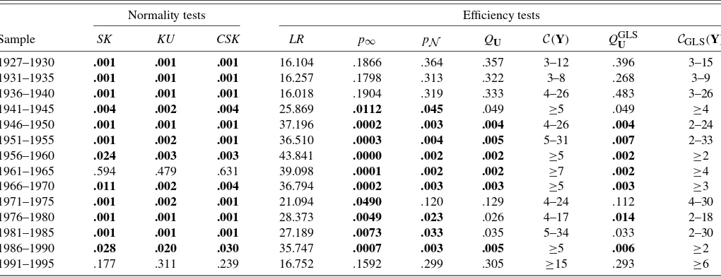
Table 1 reports tests of the unconditional CAPM over 5-year subperiods. We also ran the analysis with 10-year subperiods; the results are not significantly affected by such modifications. A notable feature emerges from Table 1: Test decisions (cerning MLR errors and the zero-intercept restriction) vary con-sistently over time. Such effects are documented in empirical work on the CAPM (see Black 1993; Fama and French 2004). Indeed, temporal instabilities have motivated subperiod model analysis and spurred further research aimed at capturing time-varying betas. Our results, which allow for short time spans, reveal temporal instabilities even when accounting for non-Gaussian errors. Our analysis of the conditional model (dis-cussed later) points out to similar problems in the latter context. Table 1 reports (in columns 1–3) the p values of the ex-act multinormality tests based onESK, EKU, and CSK (see Sec. 5.1). These tests allow us to evaluate whether observed residuals exhibit non-Gaussian behavior through excess skew-ness and kurtosis. For most subperiods, normality is rejected. These results are interesting, because, although it is well ac-cepted in the finance literature that continuously compounded returns are skewed and leptokurtic, empirical evidence of non-normality is weaker for monthly data. For instance, Affleck-Graves and McDonald (1989) rejected normality in about 50% of the stocks that they studied. Our results, which are exact (i.e., cannot reject spuriously), indicate much stronger evidence
Table 1. Normality and unconditional efficiency tests
Normality tests Efficiency tests
Sample SK KU CSK LR p∞ pN QU C(Y) QGLSU CGLS(Y)
1927–1930 .001 .001 .001 16.104 .1866 .364 .357 3–12 .396 3–15
1931–1935 .001 .001 .001 16.257 .1798 .313 .322 3–8 .268 3–9
1936–1940 .001 .001 .001 16.018 .1904 .319 .333 4–26 .483 3–26
1941–1945 .004 .002 .004 25.869 .0112 .045 .049 ≥5 .049 ≥4
1946–1950 .001 .001 .001 37.196 .0002 .003 .004 4–26 .004 2–24 1951–1955 .001 .002 .001 36.510 .0003 .004 .005 5–31 .007 2–33
1956–1960 .024 .003 .003 43.841 .0000 .002 .002 ≥5 .002 ≥2
1961–1965 .594 .479 .631 39.098 .0001 .002 .002 ≥7 .002 ≥4
1966–1970 .011 .002 .004 36.794 .0002 .003 .003 ≥5 .003 ≥3
1971–1975 .001 .002 .001 21.094 .0490 .120 .129 4–24 .112 4–30 1976–1980 .001 .001 .001 28.373 .0049 .023 .026 4–17 .014 2–18 1981–1985 .001 .001 .001 27.189 .0073 .033 .035 5–34 .033 2–30
1986–1990 .028 .020 .030 35.747 .0007 .003 .005 ≥5 .006 ≥2
1991–1995 .177 .311 .239 16.752 .1592 .299 .305 ≥15 .293 ≥6
NOTE: Numbers in bold indicate test results that are significant at the .05 level. Columns 1–3 reportpvalues for multinormality tests. Columns 1 and 2 pertain to the null hypotheses of no excess skewness and no excess kurtosis in the residuals of each subperiod. Thepvalues in column 3 correspond to the combined statistic CSK designed to jointly test for the presence of skewness and kurtosis; individual and joint tests are obtained by applying (30) and (31) under the assumption of multivariate normal errors in the context of (2). Column 4 presents the quasi-LR statistic defined in (20) to testHEdefined by (1) in the context of (2); columns 5, 6, and 7 are the associatedpvalues using, respectively, the asymptotic chi-squared distribution, the corresponding (pivotal) MC test obtained under the assumption of multivariate normal errors, and a MMC test assuming a multivariatet(κ) error distribution where the pvalue is maximized over a confidence set forκwith level 1−α1=.975. In the latter case, the maximizedpvalue for the corresponding efficiency test is significant at level .05 if it is not larger thanα2=.025. The confidence set forκis reported in column 8; see Section 4 for details on its construction. Columns 9 and 10 are the GLS (weighted QMLE) counterparts of 7–8, using the variance weights (36) to correct for heteroscedasticity.
Table 2. Normality and conditional efficiency tests
Normality tests Conditional efficiency tests
Sample SK KU CSK LR p∞ pN QU C(Y)
Model (7)
1966–1970 .085 .017 .033 122.545 .0002 .111 .125 ≥4
1971–1975 .778 .986 .908 130.384 .0000 .057 .067 ≥6
1976–1980 .095 .118 .137 147.084 .0000 .012 .021 ≥4
1981–1985 .707 .095 .141 155.475 .0000 .004 .005 ≥4
1986–1990 .114 .032 .046 109.736 .0028 .300 .344 ≥3
1991–1995 .611 .501 .645 113.462 .0013 .207 .225 ≥6
1966–1995 .001 .001 .001 162.050 .0000 .001 .001 3–16
Model (5)
1966–1970 .275 .014 .025 34.344 .0006 .011 .015 ≥4
1971–1975 .093 .139 .130 26.166 .0102 .072 .087 ≥5
1976–1980 .013 .002 .001 31.903 .0014 .021 .023 ≥4
1981–1985 .019 .024 .028 32.655 .0011 .019 .026 ≥4
1986–1990 .019 .015 .028 31.932 .0014 .020 .024 ≥4
1991–1995 .160 .381 .200 17.976 .1164 .338 .347 ≥11
1966–1995 .001 .001 .001 39.790 .0001 .001 .001 4–15
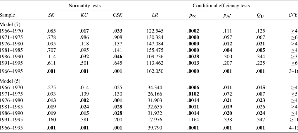
NOTE: Numbers in bold indicate test results that are significant at the .05 level. Columns 1–3 reportpvalues for multinormality tests. Columns 1 and 2 pertain to the null hypothesis of no excess skewness and no excess kurtosis in the residuals of each subperiod. Thepvalues in column 3 correspond to the combined statistic CSK designed to jointly test for the presence of skewness and kurtosis; individual and joint tests are obtained by applying (30) and (31) under the assumption of multivariate normal errors, in the context of (5) and (7). Column 4 presents the quasi-LR statistic defined in (20) to testHE1defined by (6) [for model (5)], andHE2defined by (8) [for model (7)]; columns 5, 6, and 7 are the associatedpvalues using, respectively, the asymptotic chi-squared distribution, the corresponding (pivotal) MC test obtained under the assumption of multivariate normal errors, and a MMC test assuming a multivariatet(κ) error distribution where thepvalue is maximized over a confidence set forκwith level 1−α1=.975. In the latter case, the maximizedpvalue for the corresponding efficiency test is significant at level .05 if it is not larger thanα2=.025. The confidence set forκis reported in column 8; see Section 4 for details on its construction.
against normality. This also confirms the results of Richardson and Smith (1993), who provided evidence against multivariate normality based on asymptotic tests (see also Fiorentini et al. 2003). Of course, this evidence provides further motivation for using our approach to test mean–variance efficiency under non-Gaussian errors.
Columns 4–7 of Table 1 present the LR statistics for uncon-ditional mean–variance efficiency, the corresponding asymp-toticpvalues obtained from the asymptoticχ2(n)distribution (p∞), the exact Gaussian-based MCp values (pN), and the maximized MC p values based on the Student-t error model (QU). Column 8 gives the confidence setC(Y)for the number of degrees of freedom,κ. These results show that asymptotic
pvalues are quite often spuriously significant (e.g., for 1941– 1955), and that the maximal p values exceed the Gaussian-basedpvalue. It is “easier” to reject the testable implications under normality. For instance, at the 5% level of confidence, we find 10 rejections (out of the 14 subperiods) of the null hypoth-esis for the asymptoticχ2(12)test, 9 for the MCpvalues un-der normality, and 6 unun-der the Student-tdistribution. Under the Student distribution, the testsjointlyassess the mean–variance efficiency hypothesis and the unknown degrees of freedom pa-rameters in the error distribution. Because the confidence level for the nuisance parameter is.975(α1=.025),pvalues for the efficiency tests should be compared withα2=.025 to ensure that the overall level of the test isα=α1+α2=.05; see Sec-tion 4.
These findings differ from those of Zhou (1993), who found no change in the rejection rates of mean–variance efficiency us-ing elliptical distributions other than the normal. This may be due to the fact that we explicitly take into account nuisance pa-rameter uncertainty (e.g., the fact that the degrees-of-freedom
parameter is unknown). Interestingly, whenever the results obtained under non-Gaussian distributions differ from those obtained under the Gaussian distribution, the Gaussian distri-butional assumption is strongly rejected. Our results clearly indicate that GRS-type tests are sensitive to the hypothesized error distribution. Of course, this observation is relevant when the hypothesized distributions are empirically consistent with the data. Focusing on the t distributions with parameters not rejected by exact GF tests, we see that the decision of the MMC mean–variance efficiency test can change relative to theF-based test.
It is usual to aggregate the efficiency test results over all subperiods, in some manner. For instance, Gibbons and Shanken (1987) proposed two aggregate statistics, which, in terms of our notation, may be expressed as
GS1= −2 14
j=1
ln(pN[j]) and
(39)
GS2= 14
j=1
−1(pN[j]),
where [j] refers to the subperiods and −1(·) provides the standard normal deviate corresponding topN[j]. If the mean– variance efficiency hypothesis holds across all subperiods, then
GS1∼χ2(2×14), whereas GS2∼N(0,14). It is notewor-thy that the same aggregation methods can be applied to our test problem even under (16) by replacing, in (39),pN[j]with QU[j], the MMC p values obtained imposing (16). Indeed, as is observed by Gibbons and Shanken (1987), theF-distribution is not needed to obtain the null distribution of these combined statistics. All that is needed is a continuous null distribution
(a hypothesis satisfied by normal and Student-t errors) and, of course, independence across subperiods. Our results, under normal and Student-t errors, areGS1=102.264 and 101.658 andGS2=28.476 and 28.397; the associatedpvalues are ex-tremely small. If independence is upheld, as done by Gibbons and Shanken (1987), then this implies that mean–variance ef-ficiency is jointly rejected by our data. If one questions inde-pendence and prefers to combine using Bonferroni-based crite-ria, then the smallestpvalue is .002, which, when referred to .025/14≃.002, comes close to a rejection. In the context of a MC with 999 replications, the smallest possiblepvalues are .001, .002, and so forth. To allow for a fair Bonferroni test, it is preferable to consider the level.028/14=.002. This means that in every period the pretest confidence set should be applied withα1=.022 to allow.028 to the mean–variance efficiency test. The results reported in the foregoing tables are robust to this change in level.
Finally, Table 3 presents the results of our multivariate ex-act diagnostic checks for departures from the iid assumption— namely, our proposed multivariate versions of the Engle, Lee– King, and variance ratio tests; we use 12-month lags. The re-sults show very few rejections of the null hypothesis at both the 1% and 5% levels of significance. This implies that in our sta-tistical framework and for the time spans analyzed, iid errors provide an acceptable working assumption. Our heteroscedas-ticity tests also show that analyzing mean–variance efficiency through elliptical distributional assumptions on the errors is sta-tistically valid in our sample.
An advantage of our methodology is that weighted QMLE-based tests (i.e., tests QMLE-based on weighted QMLE) may easily be conducted following the methodology that we have described herein, in the context of an MLR weighted by the necessary variance correction term, by, for example, using the variance
Table 3. Multivariate diagnostics, unconditional CAPM
Normal errors Student-terrors
Sample E˜ LK VR E˜ LK VR BP
1927–1930 .001 .356 .004 .013 .301 .004 .285 1931–1935 .022 .748 .069 .082 .659 .066 .016 1936–1940 .075 .612 .855 .124 .587 .867 .087 1941–1945 .824 .979 .163 .843 .982 .177 .034 1946–1950 .003 .804 .063 .017 .784 .068 .880 1951–1955 .139 .353 .111 .168 .321 .120 .591 1956–1960 .987 .628 .093 .994 .628 .095 .347 1961–1965 .339 .207 .577 .375 .195 .584 .771 1966–1970 .027 .274 .821 .043 .278 .847 .961 1971–1975 .280 .224 .218 .316 .212 .224 .013 1976–1980 .004 .011 .165 .016 .013 .183 .406 1981–1985 .027 .103 .208 .050 .103 .217 .583 1986–1990 .033 .453 .346 .077 .442 .366 .279 1991–1995 .803 .236 .088 .821 .252 .092 .585
NOTE: Numbers shown arepvalues associated with the combined testsE˜,LK, andVR
defined by (35), in the context of model (2).E˜andLKare multivariate versions of Engle’s and Lee–King’s GARCH tests, andVRis a multivariate version of Lo and MacKinlay’s variance ratio tests; see Section 5.2.BP[defined in (37)] is the conditional heteroscedas-ticity test as function of the benchmark returns, which is relevant for elliptical nonnormal errors; see Section 5.3. The MCpvalues in columns 1–3 are based on pivotal statistics, while those in columns 4–7 are MMCpvalues obtained by maximizing over confidence sets (with level .975) of distributional nuisance parameters. The confidence sets used are those reported in Table 1 (column 8). Numbers in bold indicate test results significant at level .05.
weights (36) in the case of the multivariate-t(see also Vorkink 2003, footnote 4) as described at the end of Section 5. For il-lustrative purposes, we report the correctedpvalues for multi-variatet-type tests, in column 9 of Table 1. Our results show that the decision of our tests is not notably affected when we correct for time-varying volatility. It is noteworthy that the lat-ter GLS-based correction does use (in some form) conditioning information.
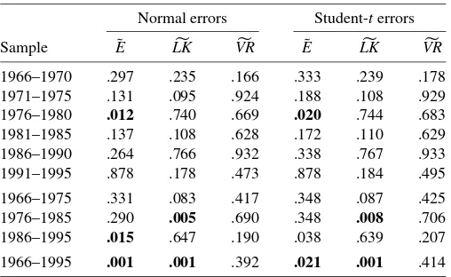
We now turn to Table 2, which reports our conditional test results for the two models (5) and (7) over 5-year intervals and over the whole sample. We retain the same layout as in Table 1, except of course that the GLS approach is no longer justified and thus is not applied in this context. The companion diagnos-tic tests are given in Table 4. Although at first glance, the sub-period analysis may appear unnecessary, given that the condi-tional model is supposed to account for time-varying betas, care must be exercised when interpreting the full-sample test results. From Table 2, we see that for both models (5) and (7): (a) the ef-ficiency hypotheses when assessed using the whole sample are soundly rejected using asymptotic or MCpvalues, (b) the con-fidence sets on the degrees-of-freedom parameter appear dra-matically tighter, and (c) normality is definitely rejected. Un-fortunately, our diagnostic tests (see Table 4) reveal significant departures from the statistical foundations underlying the latter tests (even when allowing for nonnormal errors); thus temporal instabilities cast doubt on the full-sample analysis. The tests in Table 4 are applied in the context of the conditional model (7); because the latter nests model (5) and the unconditional model as well, the results of Table 4 indicate temporal instabilities for all three models.
When we move to subperiod analysis, which appears to be appropriate in the present context, we see that the test results do not differ considerably from the unconditional case. First, as-ymptoticpvalues are quite often spuriously significant, particu-larly in the case of model (7); indeed, as may be seen in Table 2, there is a large difference between the asymptotic and the MC
Table 4. Multivariate diagnostics, conditional CAPM
Normal errors Student-terrors
Sample E˜ LK VR E˜ LK VR
1966–1970 .297 .235 .166 .333 .239 .178 1971–1975 .131 .095 .924 .188 .108 .929 1976–1980 .012 .740 .669 .020 .744 .683 1981–1985 .137 .108 .628 .172 .110 .629 1986–1990 .264 .766 .932 .338 .767 .933 1991–1995 .878 .178 .473 .878 .184 .495
1966–1975 .331 .083 .417 .348 .087 .425 1976–1985 .290 .005 .690 .348 .008 .706 1986–1995 .015 .647 .190 .038 .639 .207
1966–1995 .001 .001 .392 .021 .001 .414
NOTE: Numbers shown arepvalues associated with the combined testsE˜,LK, andVR, defined by (35), in the context of model (5).E˜andLKare multivariate versions of Engle’s and Lee–King’s GARCH tests, andVRis a multivariate version of Lo and MacKinlay’s variance ratio tests; see Section 5.2.BP[defined in (37)] is the conditional heteroscedas-ticity test as function of the benchmark returns, which is relevant for elliptical nonnormal errors. The MCpvalues in columns 1–3 are based on pivotal statistics, whereas those in columns 4–11 are MMCpvalues obtained by maximizing over confidence sets (with level .975) of distributional nuisance parameters. The confidence sets used are those reported in Table 2 (column 8). Numbers in bold indicate test results which are significant at the .05 level.
(Gaussian and non-Gaussian)pvalues. Of course, the number of restrictions tested in this case is 6 per equation (globally, 72 constraints), whereas the problem of testing intercepts involves 12 constraints. Also note that the expanded regression includes 12 regressors for 12 equations, so the number of “effective ob-servations” available for the test is quite small. This observation may suggest that power considerations underlie our observed nonrejections for the shorter subsample, although the simula-tion studies reported by Dufour and Khalaf (2002b) indicate very good power properties for sample sizes as small as 25 ob-servations even in high-dimensional MLR models. Recall that an F-test (of the GRS type) is unavailable for model (7), so our MC exact test approach is quite useful even given Gaussian errors. Similar considerations hold for the diagnostic tests: sim-ulation results reveal good power for samples of sizes compa-rable to those used in this article, especially when the system involves a large number of equations (see Dufour et al. 2005).
Second, as in the unconditional case, the Student-t maxi-mal p values exceed the Gaussian p value. For instance, for model (5), at the 5% significance level, we find five rejections (out of the six subperiods) of the null hypothesis for the asymp-totic test, four for the MC test under normality, and three under the Student-tdistribution. For model (7), at the 5% significance level, we find six rejections (out of the six subperiods) of the null hypothesis for the asymptotic test and two for the MC test under normality and the Student-tdistribution. Not surprisingly, in the subperiods in which the conditional models are rejected, the unconditional model is also rejected. In general, model (7) is rejected in fewer subperiods relative to model (5) and the un-conditional model (over the 1966–1995 subsample, where the data allow estimation of the conditional models).
In the case of (7), it might be useful to assess the significance of the intercepts only or, alternatively, to assess the contribution of the instruments in explaining excess returns. Interestingly, the MCpvalues for our test on the intercepts for the six subpe-riods are .759, .933, .075, .318, .617, and .485 under normality and .771, .946, .080, .339, .645, and .519 givent-errors. We thus see that at the 5% level, our rejections of efficiency are driven by the significance of instruments.
In view of time instabilities, the conditional efficiency test applied to the full sample is unreliable. Thus, to aggregate our subperiod analysis, once again we resort to the combined sta-tistics used by Gibbons and Shanken (1987) as in the uncon-ditional case. Our results, under normal and Student-t errors are [pvalues are reported in brackets]GS1=35.572 [.00038] and 33.006 [.00097] and GS2 =9.052 [.00011] and 8.415 [.00029] for model (7), andGS1=39.572 [.00001] and 37.703 [.00017] andGS2=10.331 [.00000] and 9.839 [.00000] for model (5). The latter p values imply that mean–variance ef-ficiency is jointly rejected with our data. Once again, if we question independence and prefer to combine using Bonferroni-based criteria, then the smallestpvalue for (7) is .004 under nor-mality and .005 witht-errors; the latter, when compared with .025/6≃0.004, comes close to a rejection. Efficiency on the aggregate in model (5) fails to be rejected by the Bonferroni rule. Viewed collectively, our subperiod and aggregate tests in-dicate that the method used to incorporate conditioning infor-mation has nonnegligible implications on mean–variance effi-ciency.
These results motivate the use of alternative models that cap-ture conditioning information in more parsimonious approaches (i.e., with fewer degrees-of-freedom losses). Inevitably, such approaches, as well as nonlinear stochastic discount factor– based models, will lead to instrumental variable contexts (see the foregoing references on GMM-based tests of the CAPM), for which the literature on exact testing is still scarce.
7. CONCLUSION
In this article we have proposed exact mean–variance ef-ficiency tests in the context of unconditional and conditional CAPMs with Gaussian or non-Gaussian disturbances. We have also shown how to deal with—in finite samples—Student-t er-rors which may involve unknown parameters. Our empirical results clearly show that the normality assumption does not fit CAPM error returns, even for monthly data. In contrast, Student-t distributions appear to be consistent with the data. Exact unconditional mean–variance efficiency tests, which for-mally account for nonnormality, fail to reject efficiency for three out of nine subperiods for which Gaussian-based tests are significant. The conditional models analyzed herein pro-vide a better fit, but the efficiency restrictions are rejected for at least half of the six subperiods considered. The conditional results are notably sensitive to the method used to incorporate conditioning information. Overall, although mean–variance ef-ficiency is rejected for several subperiods, using finite-sample methods and allowing for nonnormal errors reduces the number of subperiods for which efficiency is rejected and the strength of the evidence against it.
Although we focused here on mean–variance efficiency tests, it is noteworthy that the proposed methodology applies to sev-eral interesting asset pricing tests, including problems in which Hotelling’s test (exploited by GRS and MacKinlay 1987) and Rao’sFtest (see Stewart 1997; Dufour and Khalaf 2002b, the app.) have been used. In view of its fundamental importance, mean–variance efficiency is one of the few MLR-based prob-lems that have been approached from an exact perspective in econometrics, but some authors have recognized that hypothe-ses dealing with the joint significance of the coefficients of two regression coefficients across equations can also be tested by applying Rao’s F test. Examples include intertemporal asset pricing tests by Shanken (1990, footnote 18). Furthermore, as discussed by Shanken (1996), econometric tests of spanning also fall within this class. Indeed, spanning tests (see the sur-vey in DeRoon and Nijman 2001) may be written in terms of a model of GRS form. However, the hypothesis is more restric-tive in the sense that, in addition to the restrictions on the in-tercepts, the betas of each regression must sum to 1. These hy-potheses fit into our UL framework. Alternatively, assessing the significance of squared market returns in the context of a three-moment asset pricing model (see, e.g., Barone-Adesi, Gagliar-dini, and Urga 2004) can be carried out using our framework. The results in this article extend available exact tests of these important financial problems beyond the Gaussian context.
The fact remains that the results presented in this article are specific to UL hypotheses. Not all linear hypotheses may be cast in this form. In earlier work (Beaulieu, Dufour and Khalaf 2005), we studied extensions to nonlinear problems, including
tests of mean–variance efficiency in the context of Black’s ver-sion of the CAPM. Finally, we note that an apparent shortcom-ing of our exact tests comes from the fact that the right-side benchmark may be observed with errors. The development of exact tests that correct for errors-in-variables problems also ap-pears to be an important issue, and we are currently pursuing research on it.
ACKNOWLEDGMENTS
The authors thank Christian Gouriéroux, Raymond Kan, Blake LeBaron, Mathilda Yared, Guofu Zhou, two anonymous referees, an associate editor, and the editor, as well as seminar participants at the 2000 EC2meetings, CREST (Paris), the Uni-versity of British Columbia, the UniUni-versity of Toronto, the 2001 Canadian Economic Association meetings, CIRANO, and the Deutsche Bundesbank for several useful comments. This work was supported by the Canada Research Chair Program (Chair in Econometrics, Université de Montréal, and Chair in Environ-mental and Financial Econometric Analysis, Université Laval), the Alexander-von-Humboldt Foundation (Germany), the Insti-tut de finance mathématique de Montréal (IFM2), the Canadian Network of Centres of Excellence (program on Mathematics of Information Technology and Complex Systems [MITACS]), the Canada Council for the Arts (Killam Fellowship), the Natural Sciences and Engineering Research Council of Canada, the So-cial Sciences and Humanities Research Council of Canada, the Fonds de recherche sur la société et la culture (Québec), and the Fonds de recherche sur la nature et les technologies (Québec). This article was also partly written at the Centre de recherche en Économie et Statistique (INSEE, Paris) and the Institut für Wirtschaftsforschung Halle (Germany).
APPENDIX: TESTS
This appendix summarizes the MC test method (given a right-tailed test) as it applies to the test statistics considered in this article. (For proofs and references, see Dufour 2006.)
A.1 Monte Carlo Tests
LetS(y,X)be a test statistic that can be rewritten in the form
S(y,X)= ¯S(W,X) (A.1)
under the null hypothesis, whereWis defined by (16) and the distribution ofWis known. For example,S(y,X)could be the LR statistic considered in Theorem 1. Then the conditional dis-tribution ofS(y,X), givenX, is completely determined by the matrixXand the conditional distribution ofWgivenX; that is,
S(y,X)is pivotal. We can then proceed as follows to obtain an exact critical region:
1. LetS(0)be the observed test statistic (based on data). 2. By Monte Carlo methods, draw N iid replications of
W:W(j)= [W(j) 1 , . . . ,W
(j)
n ],j=1, . . . ,N.
3. From each simulated error matrixW(j), compute the sta-tistics S(j) = ¯S(W(j),X),j=1, . . . ,N. For instance, in the case of the QLR statistic underlying Theorem 1, cal-culateL(W(j))=Tln(|W′
(j)M0W(j)|/|W′(j)MW(j)|),j= 1, . . . ,N.
4. Compute the MCpvaluepˆN[S] ≡pN(S(0),S), where
pN(x,S)≡
NGN(x,S)+1
N+1 (A.2)
and
GN(x,S)≡
1
N
N
j=1
I[0,∞)
S(j)−x,
I[0,∞)(x)=
1 ifx∈ [0,∞)
0 ifx∈ [/ 0,∞). (A.3)
In other words,pN(S(0);S)= [NGN(S(0);S)+1]/(N+1),
whereNGN(S(0);S)is the number of simulated values that
are greater than or equal toS(0). WhenS(0),S(1), . . . ,S(N) are all distinct [an event with probability 1 when the vec-tor(S(0),S(1), . . . ,S(N))′has an absolutely continuous dis-tribution],RˆN(S(0))=N+1−NGN(S(0);S)is the rank of
S(0)in the seriesS(0),S(1), . . . ,S(N).
5. The MC critical region ispˆN[S] ≤α,0< α <1. Ifα(N+
1)is an integer and the distribution ofSis continuous un-der the null hypothesisHE, then, underHE,
PpˆN[S] ≤α
=α. (A.4)
The foregoing algorithm is valid for any fully specified dis-tribution of W. Now consider the case in which the distribu-tion ofWinvolves a nuisance parameter as in (16). In this case, givenν, (A.2) yields an MCpvalue that we denote bypˆN[S|ν],
where the conditioning on ν is emphasized for further refer-ence. The test defined bypˆN[S|ν] ≤αhas sizeα[in the sense
of (A.4)] for knownν.Treatingν as a nuisance parameter, the test based on
sup ν∈0 ˆ
pN[S|ν] ≤α, (A.5)
where0 is a nuisance parameter set consistent withHE, is
exact at levelα(see Dufour 2006). Note that no asymptotic ar-gument on the numberNof MC replications is required to ob-tain the latter result; this is the fundamental difference between the latter procedure and the (closely related) parametric boot-strap method, which in this context would correspond to a test based onpˆN[S| ˆν0], whereν0ˆ is any point estimate ofν. In earlier
work (Dufour and Khalaf 2002b), we call the test based on sim-ulations using a point nuisance parameter estimate a local MC (LMC) test. The term “local” reflects the fact that the underly-ing MCpvalue is based on a specific choice for the nuisance parameter. Furthermore, we show that LMC nonrejections are exactly conclusive in the following sense: IfpˆN[S| ˆν0]> α, then the exact MMC test is clearly not significant at levelα.
A.2 MC Skewness and Kurtosis Tests
The algorithm for implementing the MC skewness and kurto-sis tests can be decomposed in three wide steps. A more detailed discussion has been given by Dufour et al. (2003).