HUMAN CAPITAL VERSUS THE SIGNALING HYPOTHESES:
THE CASE OF INDONESIA
Nenny Hendajany
Faculty of Economics, Universitas Sangga Buana YPKP Bandung
(nennyhendajany@gmail.com)
Tri Widodo
Faculty of Economics and Business, Universitas Gadjah Mada
(kociwid@yahoo.com)
Eny Sulistyaningrum
Faculty of Economics and Business, Universitas Gadjah Mada
(eny@ugm.ac.id)
ABSTRACT
Education positively affects a person's income. It can be explained in two ways. Firstly, education directly increases the productivity of a person, which is in accordance with the views of the theory of human capital. The second way is an indirect effect, in which education acts as a sign (signal) of a worker’s unobserved characteristics, as assessed by an employer who is considering hiring the person. This is consistent with the view of the signaling theory. Both views are often debated in literature. This paper examines the returns to education in Indonesia, separating out the credential effects from the pure years of schooling effects. We used survey data from the Indonesian Family Life Survey (IFLS) 2000, 2007, and 2014 to test the difference of the two theories in estimating the returns to education in Indonesia. This study used three models which consisted of the human capital model, the signaling
model, and the
hybrid model. The human capital model used the number of years of
schooling as a variable representing education, the signaling model used dummy variables from the level of education achieved (elementary school, junior high school, senior high school, diploma, university), and the hybrid model combined both measures of the variables. The hybrid model allows for the separation of the impact of human capital based on an additional year of schooling, and the impact of signaling by the accomplishment of a particular certificate. The results of the study provide strong evidence of the presence of the returns to education either through the human capital or the signaling theories.Keywords: education, human capital, signaling, returns to education JEL codes: I20, J30
INTRODUCTION
The positive relationship between wages/ earnings and education in the income equation has been proven by previous research (Psacharo-poulos, 1994; Card, 1999; Selz-Laurière & Thélot, 2004). Most research has used Mincer’s specification as the basis of its modeling.1 The
1 Mincer’s specification is the equation of income associated with education and working experience (Mincer, 1974)
relationship between education and increasing wages is explained in two ways: 1) Directly, where education increases people’s productivity; 2) indirectly, where education is positively correlated with the nature of labor productivity that cannot be directly observed by the employer.
productivity. This learning explanation is usually related with the human capital theory. In the case of the second relationship, those with more schooling tend to earn more, is not only because schooling makes them more productive, but because schooling acts as a credential. This learning description is usually related with the screening theory. This shows that education is a signal to employers to assess the abilities of their workers (Weiss, 1995).
Economists accept the human capital and signaling theories to be the dominant explana-tions of the labor market’s returns to education. Distinguishing between these theories empiri-cally is infamously difficult (Willis, 1986). One suggested distinction between the two theories is the presence of the diploma effects, the parti-cularly high returns for completing a degree over and above completing a given amount of educa-tion (Hungerford & Solon, 1987; Belman & Heywood, 1991, 1997; Jaeger & Page, 1996; Frazis, 2002).
The most economists accept human capital theories to be explanations of the labor market’s returns to education with Mincer’s specification. The interpretation from the empirical findings using Mincer’s specification is very clear. It states that each additional year of education will increase wages to the same degree. The interpretation above is consistent with the view of the human capital theory.
Challenging this analysis are the education screening theories, which state that education is only a tool for signaling the abilities of a person which can be used in the workplace (Shabbir, 1991). Proponents of the screening theory argue that the higher income of a person who has a higher level of education really reflects an appreciation for their inherent capabilities (latent abilities) as workers, as sought by their employ-ers. Someone that has a better education tends to earn a higher salary. This is not because of their education, but because of their certificates or diplomas (Hungerford & Solon, 1987).
The discussions about the two views of the relationship between education and wages are still limited in the case of Indonesia. This motivated the authors to write this paper. The
purpose of this paper is to examine the differences of both the theories in estimating the returns to education in Indonesia. We used micro data from IFLS 3, IFLS 4, and IFLS 5 in estimating the returns. The estimation of the returns to education is made in three models used to achieve the research objectives. The results of this paper are expected to become inputs into the education policy of Indonesia.
This paper starts with the introduction, and then the literature review is in Section two. Furthermore, Section three describes the education system and the labor system in Indonesia, and Section four describes the data and a summary of the statistics. The next section discusses the empirical strategy. Section six describes the results of the regression analysis, and the last section contains the conclusion.
LITERATURE REVIEW
Human capital refers to all the attributes of workers that potentially increase their productivity in all or some productive tasks (Acemoglu, 2007). The difference in human capital leads to differences in productivity, which in turn causes differences in wages. The sources of these human capital differences are innate ability, schooling, the schools’ quality and non-schooling investment, training, and pre-labor market influences (Acemoglu & Autor, 2009). Schooling is the source of human capital differences that is often used by researchers. The longer individuals go to school, the greater is their human capital. The larger the human capital is, the greater the reward is.
The marginal rate of returns to education using Mincer’s specification is the same (constant) for each additional year of education. There is no influence from a certain educational level (for example, nine years for junior high school, 12 years for high school, and 16 years for college) in the case of this constant marginal. If these conditions are not fulfilled, we can state that there is an impact from graduation, or what is known as the Sheepskin effect. This effect can also be used to test the signaling hypothesis, because the independent variable used is a dummy of a certificate at a certain level.
Layard and Psacharopoulos (1974) rejected the signaling hypothesis because they did not find evidence to support the Sheepskin prediction, where the income of graduates is higher than that of those who dropped out of school. These results were used as evidence against the signaling hypothesis. The following research generally supported the signaling hypothesis by finding evidence of the Sheepskin effect, for example Hungerford and Solon (1987) and Belman and Heywood (1991).
Hungerford and Solon (1987) and Belman and Heywood (1991) proved the existence of the Sheepskin effect in America by using the Current Population Survey (CPS). They used the common Mincer equation by treating the log linear relationship of wages and years of schooling as a spline function that is discon-tinuous at each point of the years of school graduated. They added limited variable controls to the models, such as potential experience, potential experience squared, gender and race. They used the models to estimate the Sheepskin effect with a spline function and a step function. They noticed a great unusual improvement in the relationship between income and education in a certain year, such as 12 years (high school graduates) and 16 years (university graduates). The weakness of their study was the absence of data that differentiated between graduates and dropouts. In principle, the Sheepskin effect is the difference in income between graduates of the schooling system, and those who dropped out, so that both sets of data are important.
Xiu and Gunderson (2013) used the data from the China Household Income Project (CHIP) in 1995 and 2002 to explain the education returns in China, which separated the effects of graduation from the net impact of the years of schooling. The empirical results demonstrated an increased return of education when graduating from a certain level. This research contributed to the school returns literature in China, in such a way that it can distinguish separately the impact of the productivity of human capital for each additional year of successfully completed education, with graduation signaling the achievement of a particular education level. The second contri-bution was the use of a measurement of income and working experience that was more accurate than that used in previous studies. The last contribution was to connect the returns of education in the transition circumstances which China was facing, due to its wider open market economy orientation.
EDUCATION SYSTEM AND LABOR
SYSTEM IN INDONESIA
1. Education System
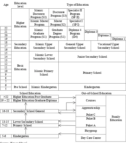
The education system in Indonesia is divided into three main types, namely formal, non-formal and informal education. Formal education is conducted in schools while non-formal and innon-formal education is conducted outside the school system. Formal education is divided into three levels, namely the basic education (primary), intermediate (secondary) and higher (tertiary). Primary education consists of elementary school or madrasah ibtidaiah and junior high school or madrasah tsanawiyah. Secondary education consists of senior high school, madrasah aliyah, and vocational school (SMK). Figure 1 illustrates the complete Indone-sian education system in accordance with the Law No. 20 of 2003. The numbers on the left side of Figure 1 shows individual average ages at a particular school level.
of Religious Affairs). Based on Law No. 20 of 2003, public schools, in either the public or private sector, are under the supervision of the Ministry of National Education, while Islamic schools, both public and private are under the supervision of the Ministry of Religious Affairs.
The informal education consists of courses, internships, Paket A, Paket B, Paket C, playgroups and childcare. The institution in charge of courses, internships, Paket A, Paket B,
and Paket C is the Ministry of National Education, while playgroups and nurseries are under the supervision of the Ministry of National Education and the Ministry of Social Affairs.
According to Law No. 20 year 2003 on the Indonesian education system, as illustrated in Figure 1, the duration of the schooling (the number of years of schooling) for each level of education is described in Table 1.
Age Education
level Type of Education
Higher Education
Islamic Doctorate Program (S3)
Doctorate Program (S3)
Specialist II Program
(SP II) Islamic Master
Program
Master Program(S2)
Specialist I (SP I) 22
Islamic Graduate Program (S1)
Graduate Degree Program (S1)
Diploma 4 Program
(D4)
21 Diploma 3
20 Diploma 2
19 Diploma 1
18
Secondary Education
Islamic Upper Secondary School
General Upper Secondary School
Vocational Upper Secondary School 17
16 15
Basic Education
Islamic Lower
Secondary School Junior Secondary School 14
13 12
Islamic Primary
School Primary School
11 10 9 8 7 6
Pre School Islamic Kindergarten Kindergarten 5
School Education Out-of-School Education >22 Higher Education Post Graduate
Courses
Family Education 19 – 22 Higher Education Graduate/Diploma
Apprenticeship
Paket C 16-18 Secondary School General
Paket B
Paket A 13-15 Lower Secondary School
7-12 Primary School
Playgroup
5-6 Kindergarten
Day Care Center
Source: Kemendiknas2
Figure 1. Education System in Indonesia, Law No. 20 2003
2
Table 1. Education Level and Years of Schooling
Years of schooling Education Level
6 9 12 14 16
Primary School Junior High School Senior High School Diploma Degree Scholar/Master’s Degree
2. Labor System
The labor market in Indonesia, according to the definition by the Central Bureau of Statistics (Badan Pusat Statistik, BPS) described by the National Labor Force Survey (Survei Angkatan
Kerja Nasional, SAKERNAS), is divided into ten business fields. They are agricultural crops, plantations, fisheries, animal husbandry, other agricultural aspects, industrial processing, trade, services, transport, and others.
In Indonesia, many workers have low levels of education. The numbers of workers with low education levels (elementary and below) far outnumber workers with other levels of education. For example in 2013, these less educated workers consisted of more than 47 percent of the workforce (equal to 54.62 million people).
Table 2. Workers Aged 15 Years and Over Who Work According to their Attainment Education, 2011-2013 (million people)
Attainment Education 2011 2012 2013
February August February August February
(1) (2) (3) (4) (5) (6)
Elementry school and less 55.12 54.18 55.51 53.88 54.62
Junior high school 21.22 20.70 20.29 20.22 20.29
Senior high school 16.35 17.11 17.20 17.25 17.77
Vocational school 9.73 8.86 9.43 9.50 10.18
Diploma I/II/III 3.32 3.17 3.12 2.98 3.22
University 5.54 5.65 7.25 6.98 7.94
Total 111.28 109.67 112.80 110.81 114.02 Source: BPS3
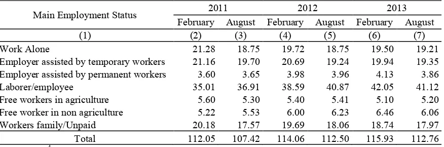
Table 3. Workers Aged 15 Years and Over Who Worked According to their Main Employment Status, 2011-2013 (million people)
Main Employment Status 2011 2012 2013
February August February August February August
(1) (2) (3) (4) (5) (6) (7)
Work Alone 21.28 18.75 19.72 18.75 19.50 19.21
Employer assisted by temporary workers 21.16 19.70 20.69 19.24 19.94 19.35 Employer assisted by permanent workers 3.60 3.65 3.98 3.96 4.13 3.86 Laborer/employee 35.01 36.91 38.59 40.87 42.05 41.12 Free workers in agriculture 5.60 5.30 5.40 5.41 5.10 5.20 Free worker in non agriculture 5.22 5.53 6.00 6.23 6.46 6.06 Workers family/Unpaid 20.18 17.57 19.69 18.06 18.74 17.97 Total 112.05 107.42 114.06 112.50 115.93 112.76 Source: BPS4
3
http://www.bps.go.id/brs_file/naker, date 8/8/2014
4
The employment status of Indonesian workers has increased. Table 3 shows Indo-nesian workers by their main employment statuses. The main employment status is the employment status of a person at his/her place of work or the establishment where he/she is employed. There are seven employment statuses based on the BPS definition. They are self-employed, self-employed with the help of temporary workers, self-employed with the help of permanent workers, laborers, agricultural free workers, non-agricultural free workers, and unpaid workers. An unpaid worker is a person who works in an establishment run by another member of the family, a neighbor or a volunteer worker, in order to earn some form of income, but not a wage.
The increase in the laborer/employee status is about 2.7 percent every year. The other increasing employment statuses are self-employed with the help of permanent workers and non-agricultural free workers. The increase in both of these is under one percent. The other employment status has decreased by an average
of less than one percent per year, and the highest decline is in the self-employed status.
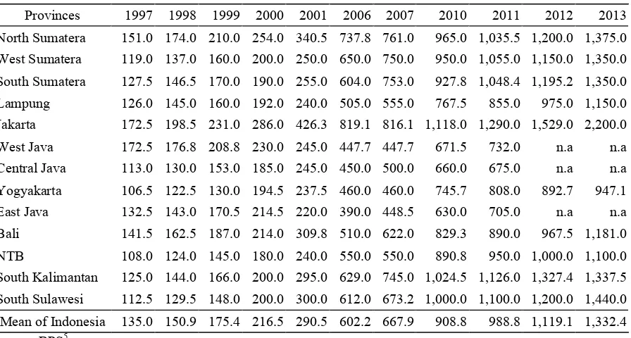
The wages in Indonesia are regulated by Law No. 13 of 2003. The income or wages of workers in Indonesia are quite varied. A regional minimum wage is used as a reference wage, although there are still many small companies or family companies paying wages below the regional minimum wage. The development of the national average minimum wage nominally increased over time. Jakarta is the province that experienced higher growth than the other provinces (Table 4).
DATA AND SUMMARY STATISTICS
Data used in this research are the IFLS data (Indonesian Family Life Survey) from 2000, 2007, and 2014. The IFLS is a large-scale longitudinal observation of individual and household levels of socio-economic status and health. The data we used were the criteria of workers aged between 15 years and 65 years old for each year surveyed, and the education level they achieved or if they no longer attend school.
Table 4 The Development of the Regional Minimum Wage 1997-2013 (In Thousand Rupiah)
Provinces 1997 1998 1999 2000 2001 2006 2007 2010 2011 2012 2013
North Sumatera 151.0 174.0 210.0 254.0 340.5 737.8 761.0 965.0 1,035.5 1,200.0 1,375.0
West Sumatera 119.0 137.0 160.0 200.0 250.0 650.0 750.0 950.0 1,055.0 1,150.0 1,350.0
South Sumatera 127.5 146.5 170.0 190.0 255.0 604.0 753.0 927.8 1,048.4 1,195.2 1,350.0
Lampung 126.0 145.0 160.0 192.0 240.0 505.0 555.0 767.5 855.0 975.0 1,150.0
Jakarta 172.5 198.5 231.0 286.0 426.3 819.1 816.1 1,118.0 1,290.0 1,529.0 2,200.0
West Java 172.5 176.8 208.8 230.0 245.0 447.7 447.7 671.5 732.0 n.a n.a
Central Java 113.0 130.0 153.0 185.0 245.0 450.0 500.0 660.0 675.0 n.a n.a
Yogyakarta 106.5 122.5 130.0 194.5 237.5 460.0 460.0 745.7 808.0 892.7 947.1
East Java 132.5 143.0 170.5 214.5 220.0 390.0 448.5 630.0 705.0 n.a n.a
Bali 141.5 162.5 187.0 214.0 309.8 510.0 622.0 829.3 890.0 967.5 1,181.0
NTB 108.0 124.0 145.0 180.0 240.0 550.0 550.0 890.8 950.0 1,000.0 1,100.0
South Kalimantan 125.0 144.0 166.0 200.0 295.0 629.0 745.0 1,024.5 1,126.0 1,327.4 1,337.5
South Sulawesi 112.5 129.5 148.0 200.0 300.0 612.0 673.2 1,000.0 1,100.0 1,200.0 1,440.0
Mean of Indonesia 135.0 150.9 175.4 216.5 290.5 602.2 667.9 908.8 988.8 1,119.1 1,332.4 Source: BPS5
5
The dependent variable used by the researcher was income per month or per year. The reason the researcher did not use income per hour was because there was no direct question that led to the income per hour in the IFLS data. The researcher needed to ask some of the other questions in the IFLS questionnaire to learn people’s income per hour. If this had been conducted, the researcher was worried that it would lead to bias caused by an error measurement. Income in this paper is the income earned from working at one’s main job. This information was obtained from the IFLS questionnaire book 3A TK section.
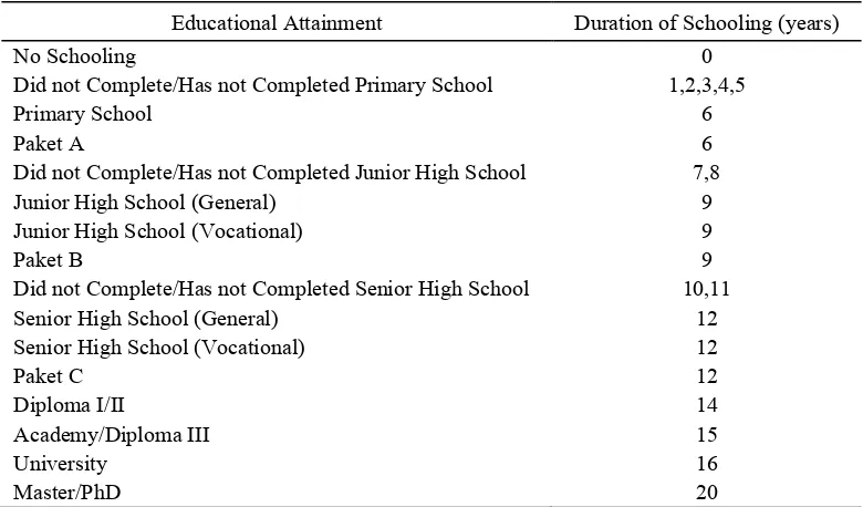
The education variable is made from two types of measurement in accordance with the two theories that we want to compare, they are the human capital theory and the signaling theory. Firstly, one measurement uses the measure of the length or duration of a person’s schooling (in years). This measurement is consistent with the human capital theory. Data of the schooling’s duration are in IFLS’s book 3A DL section. The explanation of the education’s duration in this research is in accordance with the IFLS’s questionnaire and education rules. The result is presented in Table 5.
Secondly, the other measurement uses the measure of the last certificate received (the level of the highest education completed, for example elementary, junior high school, senior high school, diploma and bachelor’s degree). This second measurement is consistent with the signaling theory. Measurement of this variable uses the dummy of the schooling’s level. Based on the data in Table 6, 19.42 percent of the respondents were people who did not graduate from elementary school. This shows that the proportion is still quite large, therefore, the researcher created a dummy for did not graduate from elementary school as the basis in the set of dummy ��(credential). The IFLS questionnaire provided an explanation about this measure with the question on DL06 and DL07.6
6
DL06 is about the highest education level attended while DL07 is about the highest grade completed at school.
The experience variable was the total number of years from starting work, measured through the (��� − ���� − �,) approach, where
��� was the age in 2000, 2007, or 2014, ����
the duration of schooling, and �, the age schooling started. The definition of experience in this case was not only working experience, but also life experience, outside of school and at the beginning of schooling. Almost all the research into returns to education used this approach. The age variable was obtained from book 3A; the duration of schooling was in accordance with the education variable, while the age schooling started was at seven years old, according to the rules governing education in Indonesia.
Control variables used in this study included the marital status of the respondents, a dummy of the city they lived in, their gender and a dummy of their employment status. Employment status was adjusted, based on the IFLS’s questionnaire, and divided into eight types: Self-employed, self-employed with help from temporary workers, self-employed with help from permanent workers, government em-ployees, private sector emem-ployees, agricultural free workers, non-agricultural free workers and unpaid workers. The researcher measured the outcome in the form of income, so the unpaid workers classification was not included as a respondent.
Table 5. Duration of Schooling
Educational Attainment Duration of Schooling (years)
No Schooling 0
Did not Complete/Has not Completed Primary School 1,2,3,4,5
Primary School 6
Paket A 6
Did not Complete/Has not Completed Junior High School 7,8
Junior High School (General) 9
Junior High School (Vocational) 9
Paket B 9
Did not Complete/Has not Completed Senior High School 10,11
Senior High School (General) 12
Senior High School (Vocational) 12
Paket C 12
Diploma I/II 14
Academy/Diploma III 15
University 16
Master/PhD 20
Note: Paket A, B, and C are for the informal school
Table 6 shows the definition of the variables used in the research and the summary statistics. The respondents who met the criteria numbered 49,001 individuals who consisted of 13,514 from IFLS3, 15,843 from IFLS4, and 19,644 from IFLS5. The average annual income of the respondent was Rp 5,789,102 with the deviation standard being Rp 7,621,662. The size of the deviation standard indicates a large inequality in incomes in Indonesia.
The average duration of education for the respondents was 8.50 years with a deviation standard of 4.44 years. Respondents who had graduated from elementary school made up 24 percent of the survey, 16 percent for junior high school, 27 percent for senior high school, 6 per-cent held a diploma and 7 perper-cent a bachelor’s degree.
Workers who held the employment status of self-employed comprised 21 percent of the respondents, self-employed with help from temporary workers made up 20 percent and self-employed with help from permanent workers were 2 percent. While workers with the employment status of government employees accounted for 8 percent and private sector employees made up 40 percent. Workers with the employment status of agricultural free
workers were 3 percent and 6 percent were in non-agricultural fields.
Based on the firms’ sizes, 57 percent of respondents worked at very small firms, small firms numbered 21 percent, medium firms accounted for 13 percent, and large firms were only 9 percent. Companies in the very small firms category were predominantly staffed by either self-employed workers or self-employed with help from temporary workers. This shows that much of the employment opportunities available to workers in Indonesia are in the informal sector, as opposed to the formal sector.
Table 6. Definition of Variables and Statistical Summary
Variable Definition of Variable Mean Standard
Deviation Min Max
Yearly earnings Individual real income from work per
year (in rupiah,2000 reference) 5,789,102 7,621,662 35,463 91,700,000 Log y Natural log of individual earnings of
work per year 14.90 1.25 10.48 18.33 University >=undergraduate university 0.07 0.25 0 1
Characteristics Age of respondents in 2007
Dummy variable male gender (Yes = 1. No = 0).
Dummy variable marital status married (Yes = 1. No = 0).
Dummy variable religion Islam (Yes = 1. No = 0).
Dummy variable individuals living in urban areas (Yes = 1. No = 0).
Dummy variable self employ-ment status (Yes = 1. No = 0).
Dummy variable self employed with unpaid family worker/tem-porary worker (Yes=1, No=0).
Dummy variable self employed with permanent worker (Yes=1, No=0). Dummy variable government worker (Yes=1, No=0).
Dummy variable private worker (Yes=1, No=0).
Dummy variable free worker in agriculture (Yes=1, No=0).
Variable Definition of Variable Mean Standard
Dummy variable lives in the province of North Sumatra (Yes = 1. No = 0) Dummy variable lives in the province of West Sumatra (Yes = 1. No = 0) Dummy variable lives in the province of South Sumatra (Yes = 1. No = 0) Dummy variable lives in the province of Lampung (Yes = 1. No = 0)
Dummy variable lives in the province of Jakarta (Yes = 1. No = 0)
Dummy variable lives in the province of West Java (Yes = 1. No = 0)
Dummy variable lives in the province of Banten (Yes = 1. No = 0)
Dummy variable lives in the province of Central Java (Yes = 1. No = 0)
Dummy variable lives in the province of Yogyakarta (Yes = 1. No = 0)
Dummy variable lives in the province of East Java (Yes = 1. No = 0)
Dummy variable lives in the province of Bali (Yes = 1. No = 0)
Dummy variable lives in the province of West Nusa Tenggara (Yes = 1. No = 0) Dummy variable lives in the province of South Kalimantan (Yes = 1. No = 0) Dummy variable lives in the province of South Sulawesi (Yes = 1. No = 0) Dummy variable lives in another province (Yes = 1. No = 0)
N Number of observation 49,001
EMPIRICAL STRATEGY
The model in this paper refers to the study of Xiu and Gunderson (2013). In our paper, we made three models that included the human capital model, the signaling model and the hybrid model. These models were used to achieve the purpose of this essay and strengthen the empirical result.
Model 1. Human capital model
This is Mincer’s basic model according to the theory of human capital. The form of the equation is:
log �2 = �,+ � ����2+ � ���2+ � ���2=+
�2� + �2,
where �2 is the income/wage of individual i.
����2 is the years of schooling completed by individual i. ���2 is the potential working experience, derived using the (age-educ-7) approach. �2 is a set of control variables that influence a person’s income. The years of schooling captures both the impact of human capital productivity from additional years of schooling as well as the impact of signaling from acquiring whatever credentials they obtained from completing key phases of their education.
Model 2. Signaling Model (credentials model) This model based on the theory of signaling/ screening. The signal used is graduating from an educational level, or the certificates possessed by the worker. This signaling model has the form of:
log �2 = �,+ ���2+ � ���2+ � ���2=+
�2� + �2
where ��is a set of dummy credential variables that reflects both the impact of human capital productivity based on additional years of schooling, as well as the impact of signaling based on acquiring whatever credentials they obtained related to completing key phases of their education. The �� set in this case is elementary, junior high school, senior high school, diploma and university.
Model 3. Hybrid model
Model 3 is the hybrid model where both the years of schooling and credentials dummy variables are included. This model takes the form:
log �2 = �,+ � ����2+ ���2+ ����2+
����2=+ �2� + �2.
This model enables us to separate the impact of human capital productivity based on addi-tional years of schooling from the impact of signaling based on acquiring specific credentials.
1. Potential Ability Bias and Error Measurement
The next potential problem is the estimation of the educational return that can be biased upwards as far as the endogenous education variable. In addition, the possibility of the estimation of the educational return also reflects unobserved factors, such as ability and moti-vation correlated with income. Some research calculates the educational return by using an instrument variable to calculate the ability bias. Most of the results are contrary to expectations about the presence of an upward bias, their research using IV tends to generate estimated values that are greater than the OLS’s tion. The literature review indicates that estima-tion is greater for educaestima-tional returns with the OLS, due to a very small ability bias (Griliches, 1977; Card, 1999). Card (1999: 1855) showed that estimations with the existing instrument variable that had been used to improve the ability bias were possible, and had a higher upward bias than the OLS’s estimations.
researchers are still much debated in the literature. The problem with the instrument in the case of Sheepskin’s analysis does not only involve the years of education, but also the various levels of education the respondents graduated from, so that the instrument’s determination is more difficult. A model made by the researcher involved five graduation variables and one education length variable, so at the very least it required six units of the instrument, each related to each decision of education that should not be associated with the omitted variable at the same time, and should not be associated with the outcome (Wooldridge, 2012: 531).
Based on the various considerations suggested above, we will not control any endogeneity in the education decision. We argue that: First, upward ability bias typically tends to be small, moreover there exists a downward bias due to the error measurement of education. Second, it is difficult to find the instrument that influences education, but does not influence income/revenue, especially in the signaling hypothesis model that involves many measures of the education variable. Third, the purpose of the research is to compare the human capital hypothesis and signaling hypothesis, so by using an instrument which is not in the three models, it may not provide a different conclusion (Xiu & Gunderson, 2013).
RESULT OF REGRESSION ANALYSIS: THE HUMAN CAPITAL MODEL, THE SIGNALING MODEL AND THE HYBRID MODEL
All three models use the natural log of income per year as the dependent variable with a control variable in accordance with the note in the table below. The result is presented in Table 7. All the models have been tested using a robust standard error and we obtained results for the error standard that were similar to those found using the OLS. Therefore, our results are presented in the table based on the OLS results.
The experience variable in these models has a diminishing effect on income. Because the coefficient of experience is positive, and the
coefficient of experience squared is negative, this equation literally implies that, for low values of experience, any additional experience has a positive effect on income. However, at some point this effect becomes negative.
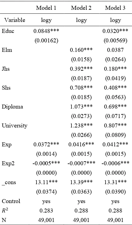
Table 7. Estimation Result
Model 1 Model 2 Model 3
Variable logy logy logy
Educ 0.0848*** 0.0320***
(0.00162) (0.00569)
Elm 0.160*** 0.0387
(0.0158) (0.0264)
Jhs 0.392*** 0.180***
(0.0187) (0.0419)
Shs 0.708*** 0.408***
(0.0185) (0.0563)
Diploma 1.073*** 0.698***
(0.0273) (0.0717)
University 1.238*** 0.807***
(0.0266) (0.0809)
Exp 0.0372*** 0.0416*** 0.0412***
(0.0014) (0.0015) (0.0015)
Exp2 -0.0005*** -0.0007*** -0.0006***
(0.0000) (0.0000) (0.0000)
_cons 13.11*** 13.39*** 13.31***
(0.0374) (0.0363) (0.0390)
Control yes yes yes
�= 0.283 0.288 0.288
N 49,001 49,001 49,001
1. Human Capital Model
Model 1 in Table 7 is a function of income based on human capital in which education is represented as the years of schooling. The result shows that each additional year of education is associated with an increase in wages of 8.48 percent for the wages per year. The experience variable (exp) is a part of the control variable that provides an impact on an increase in income by 3.72 percent for first additional year of experience. This model provides the value of �=
as being 28.3 percent.
2. Signaling Model
Model 2 in Table 7 is the signaling model, where education is represented as a set dummy of the education level variable. Respondents who did not graduate from elementary school are used as the basis of this dummy. The estimation result indicates that each school level has a positive impact on income, and the higher the level of education obtained, the greater the impact is. For example, for the model with annual income, the respondents who graduated from elementary school have a 16 percent higher income than the respondents who did not graduate from elementary school. Incomes for the graduates from junior high school are 39.2 percent higher than for who did not graduate from elementary school. The income of graduates from senior high school is 70.8 percent higher than that of those who did not graduate from elementary school. The income of graduates with diploma is 107.3 percent higher than that of those who did not graduate from elementary school. Those graduates having bachelor’s degrees and above have income that are 123.8 percent higher than those who did not graduate from elementary school.
Model 2 has 0.5 percent of the value of �=, which is higher than in the first model. This result indicates that both of the models have relatively equal strength. This shows that edu-cation in Indonesia also improves productivity. It can also be used as a signal to employers to look for the abilities of their prospective employees.
3. Hybrid Model
The hybrid model is Model 3 in Table 7, where the education level is measured by the number of years of education and from the set of dummy credentials. The result shows that the impact of the number of years of education on annual incomes is 3.2 percent. This shows that the hypothesis of human capital is significant, although the impact is smaller than when using Model 1. Graduates of elementary schools in the equation of income per year are not significant, which indicates that the certificate for the completion of elementary school is not enough to increase incomes. While the graduates of junior high school, senior high school, and diploma, or degree holders in the equation are significant. The higher the level of education, the greater the changes are in the income level. This is consistent with the hypothesis of signaling.
CONCLUSION
The hypothesis of human capital in the first model is very significant, where each additional year of education can increase the annual income by 8.48 percent. The hypothesis of signaling in Model 2 also provides a very significant result, where the higher the level of education obtained, the greater is the additional income that can be earned.
The hybrid model explains the impact of human capital that is seen from each additional year of education increasing the potential annual income by 3.2 percent, while the impact of signaling can be seen from the gaining of certificates, which is significant at the junior high school level and above. Based on the model, it can be concluded that education provides strong evidence to the equation for income, either viewed from the human capital theory aspect or the signaling theory aspect. Returns of years of schooling completed have smaller values on the hybrid model than on the human capital model, this is due to the existence of the returns of schooling level’s dummy.
incomes than an individual who does not attend or complete any level of schooling. However, the hybrid model, with the dependent variable of income per year, is significant at the junior high school level and above. The implication of this policy that can be concluded from this result is that a primary education contributes to higher productivity than an intermediate education or above. This result can be a suggestion to the government to allocate more funds to basic education programs than for intermediate education or above. In addition, it can be used as the basis of empirical evidence for giving the suggestion to the government to declare an increase from 9 years compulsory education to 12 years compulsory education.
Another conclusion that can be drawn is that there is strong evidence that workers should invest in education, due to the increased productivity they gain from it, and the difference it makes to their salaries. The role of education in both the human capital theory and the signaling theory influences individuals’ decisions to invest in their education.
REFERENCES
Acemoglu, D., 2007. Introduction to Modern Economic Growth: Part 1-5.
Acemoglu, D. and D. Autor, 2009. "Lectures in labor economics." Unpublished manuscript, Department of Economics, Massachusetts Institute of Technology, Cambridge, MA.
Available at: http://economics.mit.edu/ files/4689.
Belman, D. and J. S. Heywood, 1991. "Sheepskin effects in the returns to education: An examination of women and minorities." The Review of Economics and Statistics: 720-724.
Belman, D., & Heywood, J. S., 1997. Sheepskin Effects by Cohort: Implications of Job Matching in a Signaling Model. Oxford Economic Papers, 49(4), 623-637. doi: 10.2307/2663696
Card, D., 1999. "The Causal Effect of Education on Earnings." Handbook of labor economics 3: 1801-1863.
Frazis, H., 2002. "Human Capital, Signaling, and the Pattern of Returns to Education." Oxford Economic Papers 54(2): 298-320.
Griliches, Z., 1977. "Estimating the returns to schooling: Some econometric problems." Econometrica: Journal of the Econometric Society: 1-22.
Hungerford, T. and G. Solon, 1987. "Sheepskin Effects in the Returns to Education." The Review of Economics and Statistics 69(1): 175-177.
Jaeger, D. A. and M. E. Page, 1996. "Degrees Matter: New Evidence on Sheepskin Effects in the Returns to Education." The Review of Economics and Statistics 78(4): 733-740.
Layard, R. and G. Psacharopoulos, 1974. "The Screening Hypothesis and the Returns to Education." Journal of Political Economy 82(5): 985-998.
Mincer, J., 1974. Schooling, Experience, and Earnings, Columbia University Press. Psacharopoulos, G., 1994. "Returns to
investment in education: A global update." World development22(9): 1325-1343. Selz-Laurière, M. and C. Thélot, 2004. "The
returns to education and experience: Trends in France over the last thirty-five years." Population (english edition)59(1): 9-48. Shabbir, T., 1991. "Sheepskin effects in the
returns to education in a developing country." The Pakistan Development Review: 1-19.
Weiss, A., 1995. Human Capital vs. Signalling Explanations of Wages. The Journal of Economic Perspectives, 9(4), 133-154. doi: 10.2307/2138394
Willis, R.J., 1986. 'Wage determinants: a survey and reinterpretation of human capital earnings functions', in 0. Ashenfelter and R. Layard (eds), Handbook of Labor Economics, 1, North Holland, New York
Wooldridge, J., 2012. Introductory econo-metrics: A modern approach, Cengage Learning.
APPENDIX
(1) (2) (3)
VARIABLES Log y Log y Log y
Educ 0.0848*** 0.0320***
(0.00162) (0.00569)
Elm 0.160*** 0.0390
(0.0158) (0.0264)
Jhs 0.392*** 0.180***
(0.0187) (0.0419)
Shs 0.709*** 0.409***
(0.0185) (0.0563)
Diploma 1.074*** 0.699***
(0.0273) (0.0717)
University 1.239*** 0.808***
(0.0266) (0.0809)
Exp 0.0372*** 0.0417*** 0.0413***
(0.00144) (0.00146) (0.00146)
Exp2 -0.000533*** -0.000665*** -0.000646***
(0.0000) (0.0000) (0.0000)
Marriage 0.229*** 0.218*** 0.218***
(0.0134) (0.0133) (0.0133)
Sex 0.327*** 0.352*** 0.348***
(0.0104) (0.0104) (0.0104)
Islam -0.0539*** -0.0376* -0.0354*
(0.0207) (0.0206) (0.0206)
City 0.199*** 0.203*** 0.199***
(0.0111) (0.0110) (0.0111)
Small_firm 0.133*** 0.122*** 0.123***
(0.0140) (0.0140) (0.0140)
Medium_firm 0.329*** 0.306*** 0.306***
(0.0172) (0.0172) (0.0172)
Big_firm 0.621*** 0.608*** 0.609***
(0.0185) (0.0185) (0.0185)
Sta_2 0.261*** 0.265*** 0.263***
(0.0150) (0.0149) (0.0149)
Sta_3 0.908*** 0.891*** 0.889***
(0.0344) (0.0345) (0.0345)
Sta_4 0.580*** 0.503*** 0.500***
(0.0216) (0.0220) (0.0220)
Sta_5 0.129*** 0.122*** 0.124***
(0.0145) (0.0144) (0.0144)
Nortsumatra -0.313*** -0.296*** -0.300***
(0.0257) (0.0256) (0.0256)
Westsumatra -0.266*** -0.258*** -0.263***
(0.0280) (0.0280) (0.0280)
Southsumatra -0.309*** -0.311*** -0.315***
(0.0292) (0.0291) (0.0291)
Lampung -0.344*** -0.335*** -0.338***
Westjava -0.239*** -0.247*** -0.245*** (0.0202) (0.0201) (0.0201)
Banten -0.0554* -0.0594** -0.0574*
(0.0300) (0.0300) (0.0300)
Centraljava -0.530*** -0.535*** -0.532***
(0.0216) (0.0215) (0.0215)
Yogyakarta -0.567*** -0.573*** -0.575***
(0.0260) (0.0259) (0.0259)
Eastjava -0.330*** -0.341*** -0.338***
(0.0211) (0.0210) (0.0210)
Bali -0.205*** -0.216*** -0.210***
(0.0315) (0.0313) (0.0313)
Westnuteng -0.382*** -0.415*** -0.409***
(0.0261) (0.0260) (0.0260)
Southkalimantan -0.0265 -0.0337 -0.0357
(0.0286) (0.0285) (0.0285)
Southsulawesi -0.374*** -0.393*** -0.389***
(0.0297) (0.0297) (0.0296)
Others 0.198*** 0.195*** 0.195***
(0.0391) (0.0389) (0.0389)
T1 0.104*** 0.107*** 0.105***
(0.0121) (0.0120) (0.0120)
T2 0.344*** 0.352*** 0.349***
(0.0123) (0.0122) (0.0122)
Constant 13.11*** 13.38*** 13.30***
(0.0374) (0.0363) (0.0389)
Observations 49,001 49,001 49,001
R-squared 0.284 0.289 0.289