SPATIOTEMPORAL ANALYSIS OF URBAN LAND COVER CHANGES IN KIGALI,
RWANDA USING MULTITEMPORAL LANDSAT DATA AND LANDSCAPE METRICS
Theodomir Mugiraneza1, 2* Jan Haas3 and Yifang Ban1
1 Division of Geoinformatics, Department of Urban Planning and Environment, KTH Royal Institute of Technology, Stockholm, Sweden; [email protected]
2 Centre for Geographic Information Systems and Remote Sensing, College of Science and Technology, University of Rwanda, Huye, Rwanda; [email protected]
3 Department of Environmental and Life Sciences, Geomatics, Faculty of Health, Science and Technology, Karlstad University, Karlstad, Sweden; [email protected]
KEYWORDS: Landsat imagery, Urbanization, Land cover change, Landscape metrics, Kigali, Rwanda
ABSTRACT
Mapping urbanization and ensuing environmental impacts using satellite data combined with landscape metrics has become a hot research topic. The objectives of the study are to analyze the spatio-temporal evolution of urbanization patterns of Kigali, Rwanda over the last three decades (from 1984 to 2015) using multitemporal Landsat data and to assess the associated environmental impact using landscape metrics. Landsat images, Normalized Difference Vegetation Index (NDVI), Grey Level Co-occurrence Matrix (GLCM) variance texture and digital elevation model (DEM) data were classified using a support vector machine (SVM). Eight landscape indices were derived from classified images for urbanization environment impact assessment. Seven land cover classes were derived with an overall accuracy exceeding 88% with Kappa Coefficients around 0.8. As most prominent changes, cropland was reduced considerably in favour of built-up areas that increased from 2,349 ha to 11,579 ha between 1984 and 2015. During those 31 years, the increased number of patches in most land cover classes illustrated landscape fragmentation, especially for forest. The landscape configuration indices demonstrate that in general the land cover pattern remained stable for cropland but it was highly changed in built-up areas. Satellite-based analysis and quantification of urbanization and its effects using landscape metrics are found to be interesting for grassroots and provide a cost-effective method for urban information production. This information can be used for e.g. potential design and implementation of early warning systems that cater for urbanization effects.
1. INTRODUCTION
Since the middle of the twenty first century, unprecedented increase of urban population has been worldwide experienced. In 1950, 30% of the world’s population was urban and 66% of the world’s population is projected to be urban by 2050 (United Nations, 2015). The urbanization phenomenon is continually resulting in land use conversion for accommodating new urban structures. Globally, more than 5.87 million km2 of land have a positive probability of being converted into urban areas by 2030 (Seto et al., 2012) and it is expected that approximately 14 million hectares of arable land in developing countries will be converted for urban purposes from 1990 to 2020 (Rosegrant et al., 1997). Therefore, monitoring spatio-temporal urban growth patterns is paramount for supporting controlled urban development and satellite based data are potential for such kind of monitoring. A growing body of literature found the combination of spatio-temporal satellite data and landscape metrics (LM) worthwhile in urban land cover change analyses and environmental impact assessment (Aguilera et al., 2011; Furberg & Ban, 2010, 2012; Haas & Ban, 2014; Haas et al., 2015; Herold et al., 2005; Herold et al., 2003; Huang et al., 2007; Kuffer & Barrosb, 2011; Liu & Yang, 2015; Seto & Fragkias, 2005). However, few case studies deriving landscape indices based on satellite data exist for Sub-Saharan African cities, giving impetus for the proposed study. The remainder of this paper is structured as follows: Section 2 is dedicated to the previous works, whilst section 3 describes data used and the study area. The methodological approach is discussed in section 4. In Section 5, the analysis and discussion of the results is
presented in detail. Section 6 concludes the study and lists some 1lines of future research direction.
2. RELATED WORKS
Spatio-temporal urbanization analysis and environmental impact assessment involving the combination of remote sensing products has become a hot research topic in the last fifteen years and important literature was inventoried. Fichera et al. (2012) carried out a change detection analysis in Avellino, Italy from 1954 to 2004 using multi-source imagery including aerial photographs, ancillary data and Landsat images. Local urban landscape patterns using landscape metrics were investigated by same authors for evaluating landscape indices measured along the two transects (W-E and SW-NE directions) converging in the core urban area of the Avellino City. Haas and Ban (2014) evaluated urbanization and associated environmental impacts in China's three largest and most important urban agglomerations: Jing-Jin-Ji, the Yangtze River Delta and the Pearl River Delta. They determined urban indices for quantifying urban expansion based of classified Landsat and HJ-1A/B images. Classified remotely sensed images were further transformed into ecosystem services and a monetary approach was investigated to determine changes in ecosystem service values in the study area. Furberg and Ban (2012) studied urban land cover change detection using pixel-based Support Vector Machine classification in the Greater Toronto Area (GTA), Canada between 1985 and 2005. Landscape metrics analysis was performed based on classified Landsat images for characterizing the landscape patterns in the GTA. Interestingly, a comparative
study on satellite monitoring of urbanization between Stockholm, Sweden and Shanghai, China was conducted by (Haas et al., 2015) using Landsat images from 1989 to 2010. The impact of urbanization on ecosystem services supply was investigated and a monetary approach was used for quantifying the value of ecosystem services in the study areas. Herold et al. (2003) applied objected-oriented images analysis on very high resolution images (IKONOS and QuickBird) coupled with texture analysis for land cover assessment in Santa Barbara, California, USA. Similarly, the spatial and temporal dynamics of urban sprawl in Guangzhou, China was characterized by (Yu & Ng, 2007) by combining Landsat TM images, landscape metrics and an urban–rural gradient analysis along two selected transects. Post-classification land cover change detection analysis using multitemporal Landsat images was carried out by (Yuan et al., 2005) in seven-county Twin Cities Metropolitan Area in Minnesota. Güler et al. (2007) studied land cover change in Samsun, Turkey between 1980 and 1999 using hybrid classification and post-classification on Landsat images. While analyzing the urban expansion in Isfahan, Iran between 1956 and 2006, (Soffianian et al., 2010) used Landsat images for intermediate change detection analysis in residential areas between 1975 and 2001. Zhang and Ban (2010) coupled the V– I–S model to Tasseled Cap Transformations for monitoring the impervious surface sprawl in the Great Shanghai Area, in China. The authors satisfactorily disaggregated both impervious and non-impervious surface sprawl with more than 90% overall accuracy. In East Africa, studies using Landsat data as input for urban land cover mapping are limited despite free access to raw data. However, some successful examples do exist. Typical ones include land use monitoring using multi-sensor satellite data in Nakuru, Kenya by (Mubea & Menz, 2012) and urban growth pattern and scenario development in Kampala, Uganda between 1989 and 2010 (Vermeiren et al., 2012). Furthermore, Abebe (2013) quantified urban growth patterns in Kampala, Uganda using Landsat imagery and LM. For the case of Rwanda, there are few studies that involve the use of remote sensing techniques for land cover mapping and monitoring and more studies are needed, especially in mapping highly paced urban land cover changes. Some of the remote sensing efforts include the analysis of land cover change dynamics in Kigali, Rwanda (Akinyemi et al., 2016) using Landsat images and an intensity analysis framework. Besides, Basnet and Vodacek (2015) carried out a land cover tracking study in the cloud prone Lake Kivu region by combining Landsat imagery and ancillary data.
3. STUDY AREA AND DATA DESCRIPTION 3.1. Study Area
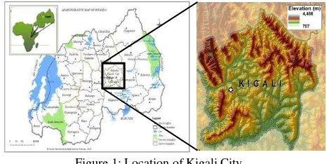
Kigali City is located in Rwanda in the Central-East African region. Geographically, it is located slightly in South of Equator at 1°56 38 S and 30°3 34 E. Kigali is Rwanda’s capital and largest city at the same time being the country’s most important business centre and main port of entry with a population estimated at 1.135 million residing in an area covering 730km2 (National Institute of Statistics of Rwanda, 2012). The city is composed of three districts namely Gasabo, Nyarugenge and Kicukiro. Figure 1 illustrates the location of Kigali within Rwanda in East African region. Land cover in the study area is composed of built-up areas fulfilling different urban functions; green space composed of forest, open vegetated land, agriculture, and wetlands. Bare lands are also found scattered throughout different corners of the city especially in the urban fringe and rural areas of the city and consist of land under
construction and uncovered soil. Water bodies composed of fish ponds, streams and part of Lake Muhazi in the extreme north of Kigali are likewise important land cover class in identified.
Figure 1: Location of Kigali City
3.2. Data Description
Land cover data was derived from three Landsat images with 30 meter resolution downloaded from the United States Geological Survey (USGS). The images with almost same anniversary dates were selected. The first Landsat-5 Thematic Mapper (TM) image was acquired on 20th June 1984, the second Landsat-7 Enhanced Thematic Mapper Plus (ETM+) image was acquired on 30 August 2001, and the third image was acquired on 12th of July 2015 using Operating Landsat Imager (OLI) on board of Landsat-8. The three images were taken with satellite track Path 172 and Row 061. A Digital Elevation Model (DEM) with 30m resolution was also acquired and included in the classification input bands. The DEM used in this study is the originated from Shuttle Radar Topographic Mission (SRTM 1) Arc-Second Global available in USGS data bank. All acquired data were projected in Universal Transverse Mercator (UTM) with the WGS-84 datum and the images were Level 1 products.
4. METHODOLOGY 4.1. Image Pre-processing
Landsat images, originally downloaded in separate files, were first stacked, thus assembling the bands into a single TIFF file. All three images were spatially subset using the study area bounding box. Linear histogram stretches and different band combinations were performed allowing on-screen visual inspection of spatial land cover distribution. The NDVI was derived from each of the three images. This was performed by rationing the red and near infrared bands (R+NIR/R-NIR) by applying the classic mathematical formula for NDVI computation (Bannari et al., 1995). Texture analysis using Gray-Level Co-occurrence Matrix (GLCM) features was performed to be integrated in the classification. Among the 14 GLCM texture measures proposed by Haralick and Shanmugam (1973), only variance was computed on Red and NIR bands. GLCM-Variance was identified as best performing texture measures while combined with spectral bands and NDVI for generally improving land cover classification accuracy (Lu et al., 2014; Shaban & Dikshit, 2001; Wentao et al., 2014) and particularly isolating formal and slum areas in urban environment (Kuffer et al., 2016). With regard to co-occurrence pixel joint probabilities calculation, the chosen direction was invariant (00) and an 11 by 11 window size was empirically determined as most suitable.
4.2. Land Cover Classification
4.2.1.Land Cover Classification Scheme
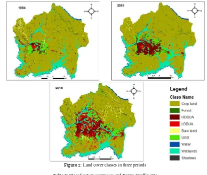
illustrated in Table 1. The shadows class was merely taken into account for practical application. Prior to landscape metrics analysis, a rural mask was applied for delineating urban green space. We hypothesized that open vegetated land localized in the core built-up zones and in the nearest urban fringe zones as urban green spaces since they are devoid of agricultural activity. This land cover category includes urban gardens, parks, golf courses, and green patches in the urban core. As a result, the landscape metrics were generated on eight land cover classes (see Figure 2).
Table 1: Land cover class description
Land cover type Description Open vegetated
land
Cultivated zones occupied with either perennial or seasonal crops, postharvest fields, pasture lands
Forest
Areas occupied by closed forest plantation with 65% canopy cover or higher, evergreen and mixed forests High-density
Built-up (HDB)
Built-up area with congested buildings, includes informal settlements
Low-density Built-up (LDB)
Built-up area with ventilation space especially high standing zones, tarmac roads, scattered settlements in urban fringe zones and in rural areas
Bare land Uncovered, permissive land/soil
Water
Permanent natural water bodies such as lakes, rivers, fish ponds reservoirs and man-made water bodies, water table in irrigated land
Wetlands
Low land with permanent water with floating aquatic vegetation especially papyrus (Cyprus papyrus), seasonal flooded low land surrounded by high lands
Shadows Shadowed zones resulting from sensors' directions
4.2.2.Training and Validation Samples Selection Both training areas and validation samples were composed of pixels randomly selected on row images using ground truth regions of interest (ROIs) in ENVI 5.3.1. A cross-checking of the corresponding landscape features in the study area was performed by referring to Google Earth. For each of the three study periods, a total number of more than five thousand pixels were selected for training areas. On the other hand, more than eight thousand pixels were chosen the validation samples for each study period. The sample size for both training and validation pixels was proportionally determined based on the size of approximate area occupied by each land cover class. However, an emphasis was put in increasing the sample size in wetlands class for avoiding pixels’ mixture given that the spectral signature was similarly confusing with open vegetated land class.
4.2.3. Support Vector Machine Classification
Pixel-based support vector machine (SVM) classification was performed using ENVI 5.3.1 after analyzing the training areas. The newly computed NDVI and GLCM bands together with the DEM were combined with the original Landsat bands 1, 2, 3, 4, 5 and 7 for Landsat TM/ETM, and bands 2, 3, 4, 5, 6 and 7 for Landsat 8 as input for SVM supervised classification at 30m resolution. The SVM classifier was selected given that it is considered as superior classification algorithm yielding good classification result. SVM is a non-parametric supervised classification algorithms based on statistical learning theory (Kavzoglu & Colkesen, 2009). In various studies, the SVM was
found as the most outperforming algorithm in improving classification accuracy comparing to other parametric and non-parametric algorithms (Foody & Mathur, 2004; Huang et al., 2002; Kavzoglu & Colkesen, 2009; Niu & Ban, 2013; Shao & Lunetta, 2012). The SVM kernel type used is Radian Basis Function (RBF) and the Gamma in kernel function was 0.1 corresponding to the inverse number of input bands. The penalty parameter together with pyramid levels and classification probability threshold were left with default values of 0, 0, and 100, respectively.
4.2.4. Post-classification Processing and Accuracy Assessment
Classification results were compared to the true information classes in the reference image. A series of post-classification clean-up operations were performed. A Sieve classes algorithm was first used for filtering the classified images which was suffering from small erroneously classified pixels. The filtering process allowed a threshold to be specified for the smallest polygon not to be merged into a neighbor. After filtering the classified image and assigning new value using Majority Analysis, land cover classes were aggregated for producing smoothed and meaningful maps. After post-classification clean-up operation, a confusion matrix was generated for accuracy assessment.
4.3. Landscape Metrics
Based on the initial classification comprising eight land cover classes, the open vegetated land class was split into the two classes including cropland and urban green spaces (UGS). Thus, landscape analysis was carried out on eight land cover class (see Figure 2) plus a shadows class which was excluded in the LM results. The UGS were delineated using urban-rural mask by taking into account the official urban administrative boundary and the urbanization indicators including dense built-up area and predominance of traffic network infrastructure.
5. RESULTS AND DISCUSSION 5.1. Land Cover Classification
Table 2 and table 3 is illustrating both the overall accuracy and Kappa Coeffient and the confusion matrices for the classified images in three considered periods (i.e. 1984, 2001, and 2015. Meanwhile table 4 represent both the producer’ and user’s accuracies. Figure 2 illustrate land cover results plus the urban green space (UGS) produced using by rural mask technique.
Figure 2: Land cover classes in three periods
Table 2: Classification accuracies and Kappa Coefficients Overall accuracy and Kappa Coefficients
1984 2001 2015
Overall accuracy 88.5% 88.6 % 93.6%
Kappa Coefficient 0.8542 0.8578 0.9177
Table 3: Producer’s and user’s accuracies (in %)
Producer's accuracies User's accuracies
No Land cover 1984 2001 2015 1984 2001 2015
1 Open land 98.8 99.8 98.4 71 73.6 80.6
2 Forest 77.1 76.6 83.1 86 97.1 85.8
3 HDB 94 97.9 98.4 96.7 92.1 98.3
4 LDB 69.5 65.5 92 96.7 92 93.2
5 Bare land 68.7 53.4 61.6 96.7 98.9 92.4
6 Water 95.5 97.6 99.6 93.4 89.8 100
7 Wetlands 84.1 87.4 93.3 97.5 97.8 98.8
The overall accuracy for 1984 classification was 88.5% with a Kappa Coefficient of 0.85. For the 2001 image, 88.6% accuracy was achieved with a Kappa Coefficient of 0.86. Similarly, the overall classification was evaluated at 93.8% with a Kappa Coefficient of 0.91 for the 2015 image. Open land was least confused with other classes in all three periods. The most difficult class to distinguish was bare land with only 53.4% accuracy in 2001, 61.6% in 2015 and 68.9% in 1984, respectively. Forests scored a good classification in 2015 with more that 80%, whilst the results were slightly worse (76.6%) in 2001 and 77.1% in 1984. In all three classified images, bare land was the most confused class where between 25% and 31% validation samples were counted as open vegetated land. The same class has also the lowest producer’s accuracy in all three periods evaluated at 53.4% in 2001, 68.7% in 1984, and 61.6% in 2015. The relative high misclassification rate in bare land is attributed to the fact its spectral signatures is very much alike that of post-harvest fields. Forests are also confused with open vegetated land where 19.7%, 22.7%, and 14.7% of class validation samples were counted as agriculture in 1984, 2001, and 2015 respectively. High commission errors were observed in 1984 in open land and forest class with 29% and 14% over-estimation. Meanwhile, the omission error is estimated at 30.5% in LDB, 31.2% in bare land and 22.9% in forest in the same period. In 2001, LDB is mostly confused either with neighboring HDB or with open vegetated land. The confusion in LDB is likely to emanate mainly from the applied threshold during post-classification operations, i.e. sieving and majority analysis and classification aggregation. In some rural areas with sloped zones contiguous to shadows, LDB are overestimated as they are spectrally interpreted as building. This was the case especially in 1984 where important scattered settlements are detected in the south-west zone. The inevitable mixed pixels in these zones neighboring shadows are attributed to the scene illumination in the hilly areas. Based on classification results, pixel-based SVM classification performed well in the complex landscape of Kigali with heterogeneous land cover expanded on hilly and shadowed terrain. The disaggregation of land cover class into sub-classes helped in avoiding overlap between classes and thus eventually misclassifications. Furthermore, GLCM (Variance) measure derived from red and NIR bands performed well in increasing land cover classes’ separability in feature space and the inclusion of DEM in classification
helped in detecting the wetland extension as depicted on Google Earth. The integration of a vegetation index band (NDVI) and a DEM into Landsat optical bands for SVM classification is believed to have contributed significantly to the good classification result as well. Particularly, the elevation data and NDVI proved effective in enhancing class separabilities and in discerning low land occupied by dry and flooded wetlands with slopes and hilly terrain.
5.2. Landscape Characteristics
The total landscape area is estimated at 73524.6 ha. Landscape is dominated by cropland in all three periods. Croplands decreased between 1984 and 2015 from 77.3% to 56.7% respectively. Forest decreased from 1400ha to 837ha between 1984 and 2001. However, forest cover increased again between intermediate and final dates with by 34.4% of the forest coverage in middle date. Built-up areas (both HDB and LDB) increased at high pace from 2 349 ha in 1984 to 11579ha in 2015. Water increased after 2001 as a result of the creation of an artificial lake in the city centre and the emergence of a lake south-east of Kigali resulting from to water rise and floods in the Nyabarongo wetlands. Other variations observed in the water class occur due to seasonal flooding in the wide Nyabarongo flood plain along the Southern border of the city landscape. Urban green spaces were manually delineated based on core urban sectors and a rural mask. Therefore, their increase in three periods is proportional to the increased of build-up areas. Furthermore, the change wetlands can be ascribed to misclassifications given that this class is confused in some locations with either cropland or forest. This is not a surprise because large parts of the wetlands are occupied by crops and because the nearest hillsides opposite the wetland are forested areas. The number of patches (NP) has increased from 1,759 in 1987 to 2,826 patches in 2015. Between 1984 and 2001, the number of patches remained almost the same (1,759 in 1984 against 1,720 in 2001). The patch density (PD) has also remained almost stable in three periods but a small incremental increase is observed from 2.3 to 3.84 patches/100ha respectively between 1984 and 2015. The largest patch index (LPI) is found in croplands that decreased almost twice between the first and last dates (77.2% in 1987 against 39.8% in 2015). The schematic representation of four investigated landscape composition indices is illustrated in Figure 3 and Figure 4.
Figure 3: Evolution of landscape composition indices
Figure 4: Evolution of landscape configuration indices
With regards to landscape configuration, it was revealed that the contrast-weighted edge density (CWED) at landscape level first decreased between initial and intermediate dates and then increased from 29meters/ha in 1984 to 40.7meters/ha in 2015. High CWED values are found in the cropland class. Furthermore, the total edge contrast index (TECI) consecutively decreasedfrom 69.9% in 1984 to 63.3% in 2001 and to 62.36% in 2015. In all three periods, the aggregation index (AI) was more than 90% at landscape level, indicating that the mosaic of patches in the landscape is generally aggregated. Nevertheless, the forest patch mosaic becomes gradually less aggregated as compared to other classes with indices evaluated at 64.1% in 1984, 63.3% in 2001 and 60.4% in 2015. Even through the built-up area was progressively replacing cropland, the latter class is still the most aggregated class with more than 95%. Figure 4 represents the evolution trends of the four analyzed landscape configuration indices from 1984 to 2015. With decreasing area and increased number of patches, forest was identified as the most fragmented class in the whole landscape especially between 1984 and 2001. This period is corresponding to the armed conflict time from 1990 to 1994 and the genocide perpetrated against the Tutsi in 1994. During that time, environmental degradation was alarming in Rwanda. Forest in particular was cut down because of massive displacement of refugees. From 2001 to 2015, forested areas increased slightly. This evolution in attributed to the government policies for environmental restoration (afforestation) especially in forest landscape (Ministry of Natural Resources, 2014). Built-up areas increased considerably after 1994 because Rwandan refugees who were living in the neighboring countries for more than four decades returned to the country, with a majority of people moving to Kigali. Other factors explaining the urban growth are rural-urban migration and natural growth rate of the population. Agriculture is the
dominating patch in the landscape that occupies more than 60% of the landscape total area in both periods, despite its reduction by almost 12%. The LPI also illustrates the
dominance of agriculture in terms of comparative patch size in the landscape.
In the present study, landscape metrics were found to be useful for spatio-temporal evaluation of the urban landscape. In Sub-Saharan African cities such as Kigali, the definition of urban circumscription is mainly guided by political decisions. It is not taking into account urban indicators such as predominance of tertiary activities, the density of built-up areas or transport networks and industries which would be amongst the driving factors for urban development. Therefore, the delineation of urban green spaces is found challenging. The urban landscape in the aforementioned sub-region is interspersed with green patches that are normally not falling in the real UGS category. Some are either used as vegetable gardens or sporadic agricultural fields. Therefore, it was necessary to delineate UGS by balancing the political boundary and the predominance of urbanization indicators (see Figure 2). In 2001, HDB are more concentrated comparing to the situation in 2015 where LDB are taking place in the old HDB (see Figure 2). This can be attributed to the fact that many tarmac roads (which were classified as LDB class) were constructed after 2001 in Kigali. The spectral signature for these roads with less than 30m width leads to classification into LDB. In addition, many areas that were informal settlements were demolished for urban redevelopment. This is the case for the commonly known Kiyovu y’Abakene (literally Kiyovu for the poor households) and Kimicanga neighborhoods. Considerable buildings were also demolished in the old central business district and high standing commercial buildings were constructed for implementing the urban master plan.
6. CONCLUSION AND FUTURE RESEARCH
that Grey Level Co-occurrence Matrix (GLCM) variance texture, vegetation index such as NDVI and elevation data such as DEM are worthwhile input for enhancing the accuracy of land cover classification especially in areas with complex and mixed land cover and hilly terrain. Landscape metrics based on classified images are also found as promising and cost effective technique for assessing and quantifying the urbanization and associated environmental impact. The vegetation index and texture analysis combined with optical Landsat bands yielded good classification results with overall classification accuracies surpassing 88% in 1984 and 2001 and 93% in 2015. Landscape composition and configuration in the last three decades were characterized using landscape metrics. It could be shown that forest and cropland were the most fragmented land cover classes and that built-up areas expanded mostly due to accelerated urbanization in the last three decades. However, the interpretation of the information derived from medium-resolution images such as Landsat could be complemented by field visits and triangulation of results with existing data which are believed to reduce misclassifications thus resulting in a more realistic classification outcome. High-resolution data is believed to further increase classification accuracies. Future research will be directed towards using mainly high-resolution satellite data, context and rule-based image classification to analyze urban land cover changes and associated environmental impact.
ACKNOWLEDGEMENTS
The research is funded by the Swedish International Development Agency (SIDA) through the SIDA-University of Rwanda Program, GIS Sub-Program, the collaborations of KTH Royal Institute of Technology, Lund University, and University of Rwanda.
REFERENCES
Abebe, GA. (2013). Quantifying urban growth pattern in developing countries using remote sensing and spatial metrics: A case study in Kampala, Uganda.
ITC Enschede, The Netherlands.
Aguilera, F, Valenzuela, LM, & Botequilha-Leitão, A. (2011). Landscape metrics in the analysis of urban land use patterns: A case study in a Spanish metropolitan area. Landscape and Urban Planning, 99(3), 226-238.
Akinyemi, FO, Pontius Jr, RG, & Braimoh, AK. (2016). Land change dynamics: insights from Intensity Analysis applied to an African emerging city.
Journal of Spatial Science, 1-15.
Ban, Y, Hu, H, & Rangel, IM. (2010). Fusion of Quickbird MS and RADARSAT SAR data for urban land-cover mapping: Object-based and knowledge-based approach. International Journal of Remote Sensing, 31(6), 1391-1410.
Bannari, A, Morin, D, Bonn, F, & Huete, A. (1995). A review of vegetation indices. Remote sensing reviews, 13(1-2), 95-120.
Basnet, B, & Vodacek, A. (2015). Tracking land use/land cover dynamics in cloud prone areas using moderate resolution satellite data: A case study in central Africa. Remote Sensing, 7(6), 6683-6709. Fichera, CR, Modica, G, & Pollino, M. (2012). Land Cover
classification and change-detection analysis using
multi-temporal remote sensed imagery and landscape metrics. European Journal of Remote Sensing, 45(1), 1-18.
Foody, GM, & Mathur, A. (2004). A relative evaluation of multiclass image classification by support vector machines. IEEE Transactions on geoscience and remote sensing, 42(6), 1335-1343.
Furberg, D, & Ban, Y. (2010). Satellite Monitoring and Impact Assessment of Urban Growth in Stockholm, Sweden between 1986 and 2006. Paper presented at the Imagin [e, G] Europe: Proceedings of the 29th Symposium of the European Association of Remote Sensing Laboratories, Chania, Greece. Furberg, D, & Ban, Y. (2012). Satellite monitoring of urban
sprawl and assessment of its potential environmental impact in the Greater Toronto Area between 1985 and 2005. Environmental management, 50(6), 1068-1088.
Gardner, RH, & O'Neill, RV. (1991). Pattern, process, and predictability: the use of neutral models for landscape analysis. Ecological Studies, 82, 289-307.
Güler, M, Yomralıoğlu, T, & Reis, S. (2007). Using landsat data to determine land use/land cover changes in Samsun, Turkey. Environmental Monitoring and Assessment, 127(1-3), 155-167.
Haas, J, & Ban, Y. (2014). Urban growth and environmental impacts in Jing-Jin-Ji, the Yangtze, River Delta and the Pearl River Delta. International Journal of Applied Earth Observation and Geoinformation, 30, 42-55.
Haas, J, & Ban, Y. (2015). Synergy of Sentenel-1A SAR and Sentenel-2A MSI data for urban ecosystem service mapping. Paper presented at the 35th EARSeL Symposium - European Remote Sensing: Progress, Challenges and Opportunities, Stockholm, Sweden, June 15-18 2015.
Haas, J, Furberg, D, & Ban, Y. (2015). Satellite monitoring of urbanization and environmental impacts—a comparison of Stockholm and Shanghai.
International Journal of Applied Earth Observation and Geoinformation, 38, 138-149. Haralick, RM, & Shanmugam, K. (1973). Textural features
for image classification. IEEE Transactions on systems, man, and cybernetics, 3(6), 610-621. Herold, M, Couclelis, H, & Clarke, KC. (2005). The role of
spatial metrics in the analysis and modeling of urban land use change. Computers, Environment and Urban Systems, 29(4), 369-399.
Herold, M, Liu, X, & Clarke, KC. (2003). Spatial metrics and image texture for mapping urban land use.
Photogrammetric Engineering & Remote Sensing, 69(9), 991-1001.
Huang, C, Davis, L, & Townshend, J. (2002). An assessment of support vector machines for land cover classification. International Journal of Remote Sensing, 23(4), 725-749.
Huang, J, Lu, XX, & Sellers, JM. (2007). A global comparative analysis of urban form: Applying spatial metrics and remote sensing. Landscape and Urban Planning, 82(4), 184-197.
Kauth, RJ, & Thomas, G. (1976). The tasselled cap--a graphic description of the spectral-temporal development of agricultural crops as seen by Landsat. Paper presented at the LARS Symposia. Kavzoglu, T, & Colkesen, I. (2009). A kernel functions
analysis for support vector machines for land cover classification. International Journal of Applied Earth Observation and Geoinformation, 11(5), 352-359.
Kuffer, M, & Barrosb, J. (2011). Urban morphology of unplanned settlements: the use of spatial metrics in VHR remotely sensed images. Procedia Environmental Sciences, 7, 152-157.
Kuffer, M, Pfeffer, K, Sliuzas, R, & Baud, I. (2016). Extraction of slum areas from VHR imagery using GLCM variance. IEEE Journal of Selected Topics in Applied Earth Observations and Remote Sensing, 9(5), 1830-1840.
Liu, T, & Yang, X. (2015). Monitoring land changes in an urban area using satellite imagery, GIS and landscape metrics. Applied Geography, 56, 42-54. Lu, D, Li, G, Moran, E, Dutra, L, & Batistella, M. (2014).
The roles of textural images in improving land-cover classification in the Brazilian Amazon.
International Journal of Remote Sensing, 35(24), 8188-8207.
Lu, D, & Weng, Q. (2006). Use of impervious surface in urban land-use classification. Remote Sensing of Environment, 102(1), 146-160.
Mahboob, MA, Atif, I, & Iqbal, J. (2015). Remote sensing and GIS applications for assessment of urban sprawl in Karachi, Pakistan. Science, Technology and Development, 34(3), 179-188.
McGarigal, K, Cushman, SA, Neel, MC, & Ene, E. (2002). FRAGSTATS: spatial pattern analysis program for categorical maps.
Ministry of Natural Resources. (2014). Forest Landscape Restoration Opportunity Assessment for Rwanda. Kigali Rwanda.
Mubea, K, & Menz, G. (2012). Monitoring land-use change in Nakuru (Kenya) using multi-sensor satellite data. Advances in Remote Sensing, 1(3), 74-84 doi:10.4236/ars.2012.13008
National Institute of Statistics of Rwanda. (2012). 2012 Population and Housing Census: Results. Kigali, Rwanda.
Niu, X, & Ban, Y. (2013). Multi-temporal RADARSAT-2 polarimetric SAR data for urban land-cover classification using an object-based support vector machine and a rule-based approach. International Journal of Remote Sensing, 34(1), 1-26.
Puissant, A, Hirsch, J, & Weber, C. (2005). The utility of texture analysis to improve per‐pixel classification for high to very high spatial resolution imagery.
International Journal of Remote Sensing, 26(4), 733-745.
Rosegrant, MW, Ringler, C, & Gerpacio, RV. (1997). Water and land resources and global food supply. Paper presented at the 1997 Conference, August 10-16, 1997, Sacramento, California.
Seto, KC, & Fragkias, M. (2005). Quantifying spatiotemporal patterns of urban land-use change
in four cities of China with time series landscape metrics. Landscape ecology, 20(7), 871-888. Seto, KC, Güneralp, B, & Hutyra, LR. (2012). Global
forecasts of urban expansion to 2030 and direct impacts on biodiversity and carbon pools.
Proceedings of the National Academy of Sciences, 109(40), 16083-16088.
Shaban, M, & Dikshit, O. (2001). Improvement of classification in urban areas by the use of textural features: the case study of Lucknow city, Uttar Pradesh. International Journal of Remote Sensing, 22(4), 565-593.
Shao, Y, & Lunetta, RS. (2012). Comparison of support vector machine, neural network, and CART algorithms for the land-cover classification using limited training data points. ISPRS Journal of Photogrammetry and Remote Sensing, 70, 78-87. Soffianian, A, Nadoushan, MA, Yaghmaei, L, & Falahatkar,
S. (2010). Mapping and analyzing urban expansion using remotely sensed imagery in Isfahan, Iran.
World applied sciences journal, 9(12), 1370-1378. United Nations. (2015). World Urbanization Prospects: The
2014 Revision: New York: United Nations Department of Economics and Social Affairs, Population Division.
Wentao, Z, Bingfang, W, Hongbo, J, & Hua, L. (2014).
Texture classification of vegetation cover in high altitude wetlands zone. Paper presented at the IOP Conference Series: Earth and Environmental Science.
Vermeiren, K, Van Rompaey, A, Loopmans, M, Serwajja, E, & Mukwaya, P. (2012). Urban growth of Kampala, Uganda: Pattern analysis and scenario development. Landscape and Urban Planning, 106(2), 199-206.
Yu, XJ, & Ng, CN. (2007). Spatial and temporal dynamics of urban sprawl along two urban–rural transects: A case study of Guangzhou, China. Landscape and Urban Planning, 79(1), 96-109. doi:http://dx.doi.org/10.1016/j.landurbplan.2006.0 3.008
Yuan, F, Sawaya, KE, Loeffelholz, BC, & Bauer, ME. (2005). Land cover classification and change analysis of the Twin Cities (Minnesota) Metropolitan Area by multitemporal Landsat remote sensing. Remote Sensing of Environment, 98(2), 317-328.
Zha, Y, Gao, J, & Ni, S. (2003). Use of normalized difference built-up index in automatically mapping urban areas from TM imagery. International Journal of Remote Sensing, 24(3), 583-594. Zhang, Q, & Ban, Y. (2010). Monitoring impervious surface
sprawl in Shanghai using tasseled cap transformation of landsat data. Paper presented at the ISPRS Technical Commission VII Symposium on Advancing Remote Sensing Science, Vienna, Austria, 5-7 July 2010.