ASSESSMENT OF THE GEOMETRIC QUALITY OF SENTINEL-2 DATA
M. Pandžić a, *, D. Mihajlović a, J. Pandžić a, N. Pfeifer b a
Faculty of Civil Engineering, Department of Geodesy and Geoinformatics, University of Belgrade, Bul. kralja Aleksandra 73, 11000 Belgrade, Serbia - [email protected], (draganm, jpandzic)@grf.bg.ac.rs
b
TU Wien, Department of Geodesy and Geoinformation, Gußhausstraße 27-29/E120.7, 1040 Vienna, Austria - [email protected]
Commission I, WG I/5
KEY WORDS: Sentinel-2, Orthophoto, Data Quality, Edge Extraction, Distance Calculation
ABSTRACT:
High resolution (10 m and 20 m) optical imagery satellite Sentinel-2 brings a new perspective to Earth observation. Its frequent revisit time enables monitoring the Earth surface with high reliability. Since Sentinel-2 data is provided free of charge by the European Space Agency, its mass use for variety of purposes is expected. Quality evaluation of Sentinel-2 data is thus necessary. Quality analysis in this experiment is based on comparison of Sentinel-2 imagery with reference data (orthophoto). From the possible set of features to compare (point features, texture lines, objects, etc.) line segments were chosen because visual analysis suggested that scale differences matter least for these features. The experiment was thus designed to compare long line segments (e.g. airstrips, roads, etc.) in both datasets as the most representative entities. Edge detection was applied to both images and corresponding edges were manually selected. The statistical parameter which describes the geometrical relation between different images (and between datasets in general) covering the same area is calculated as the distance between corresponding curves in two datasets. The experiment was conducted for two different test sites, Austria and Serbia. From 21 lines with a total length of ca. 120 km the average offset of 6.031 m (0.60 pixel of Sentinel-2) was obtained for Austria, whereas for Serbia the average offset of 12.720 m (1.27 pixel of Sentinel-2) was obtained out of 10 lines with a total length of ca. 38 km.
* Corresponding author
1. INTRODUCTION
Modern satellite missions whose aim is Earth observation provide researchers, organizations and individuals with new possibilities. In the past a decision which data to purchase involved balancing financial aspects, work to be done and timeliness of acquisition. Nowadays, when some of the distributors of satellite images have changed their distribution policy towards offering all data to the public free of charge, people do not need to worry about these issues anymore. Nevertheless, people must be aware of the restrictions of the available products not to get blindfolded by a chance of a free access to them.
To be sure that the right product is used for the right purpose, its quality assessment is necessary because any starting deviation would influence all the other subsequent products. Quality assessment is essential for Sentinel-2 orthorectified data since it is important as for any other orthophoto to be evaluated for geometric accuracy before acceptance (Greenfeld, 2001). Providers of satellite images often give very limited information about their product quality (Novák and Baltsavias, 2009). That is why testing of satellite image quality, especially by independent groups, is needed.
Assessment of geometric quality of orthophoto data can be performed in different ways. Ground Control Points (GCPs) are quite often used for testing geometric accuracy of satellite images. They can be derived either by using GPS or from large-scale controlled aerial photography (Dial et al., 2003). Another way of testing is by overlaying orthophoto onto another dataset which features better accuracy and which is, because of that,
taken as a reference. Differences in feature locations between datasets are observed and quantified, and later used for determination of the accuracy (Greenfeld, 2001). This concept is also the basis for our experiment.
One part of the experiment also deals with edge detection in order to acquire features necessary for comparison, long line segments in this case. Following (Ziou and Tabbone, 1998), most of the existing edge detectors include the three main steps: smoothing, differentiation and labeling, and the detectors differ in characteristics of each of these steps, goals, computational complexity and mathematical models used to derive them. Since the detectors differ, consequently so do the results of edge detection. Problems of edge detection are detection of false edges, missing true edges, localization, noise, etc. Operators are chosen based on the optimization of these problems. For example, operators which are good when it comes to dealing with noise are often less accurate in localization of the detected edges (Juneja and Sandhu, 2009). Whatmore, localization is affected by factors such as signal to noise ratio, observation window size and scale of smoothing filter (Kakarala and Hero, 1992).
Edge detection in the experiment was conducted by using Canny filter since visual inspection indicated better results in this case compared with using other common filters like Sobel, Prewitt's, Robert's, Laplacian of Gaussian, etc. Canny edge detection algorithm was presented in 1986 (Canny, 1986) and since then many papers confirmed its quality compared with other frequently used filters (Juneja and Sandhu, 2009, Sharifi et al., 2002). Canny technique is based on optimizing three The International Archives of the Photogrammetry, Remote Sensing and Spatial Information Sciences, Volume XLI-B1, 2016
criteria: good detection, good localization and only one response to a single edge (Basu, 2002, Ziou and Tabbone, 1998). Some papers go even further by stating that Canny edge detection algorithm performs better than other common operators under almost all scenarios (Juneja and Sandhu, 2009, Maini and Aggarwal, 2009).
2. SENTINEL-2
According to (ESA, 2015), the European Space Agency's (ESA) Sentinel-2 is high-resolution multi-spectral optical imagery satellite mission for monitoring the Earth surface. It consists of two identical satellites, Sentinel-2A and Sentinel-2B, in the same orbit phased at 180° to each other. Sentinel-2A was launched on the 23rd of June, 2015 and it features the revisit time of 10 days. When Sentinel-2B is launched (planned for mid 2016), this constellation of satellites will be able to monitor a specific area of the Earth surface every 5 days. Sentinel-2 sensors consist of 13 bands of different resolution:
• visible and near-infrared bands (4 bands in total) have
10 m resolution,
• red edge and shortwave infrared bands (6 bands in
total) have 20 m resolution and
• bands for atmospheric correction (3 bands in total)
have 60 m resolution.
Sentinel-2 images the area between 56° south and 84° north latitude. The swath width is 290 km, average altitude 786 km and mission lifetime 7 years. The orbital inclination is 98.62°. The Mean Local Solar Time at the descending node is chosen to be 10:30 (a.m.) since it provides a compromise between a minimization of a potential cloud cover, a level of solar illumination and a shadow definition (Dial et al., 2003).
As the ESA has announced, different level types of products will be available, namely:
• Level-1B, which represents Top-of-Atmosphere
radiances,
• Level-1C, which represents Top-of-Atmosphere
reflectances,
• Level-2A, which represents Bottom-of-Atmosphere
reflectances.
These products are created out of granules, in some cases also called tiles, which are the smallest indivisible partitions of a product that have all spectral bands included. Granules are of fixed size. Level-1B granules cover an area of approximately 25 × 23 km2, while Level-1C and Level-2A tiles cover an area of 100 × 100 km2. Level-1B data represents radiometrically corrected raw data, Level-1C contains applied radiometric and geometric corrections which include orthorectification and spatial registration, and Level-2A is atmospherically corrected data. The last two are in UTM/WGS84 projection. Both Level-1 products were announced to be delivered by the ESA, whereas Level-2A is to be created on the user side by using the software Sentinel-2 toolbox.
3. TEST SITE AND DATA
3.1 Austria
During satellite commissioning phase only eleven Sentinel-2 Level-1C products were available and each one covered different parts of the Earth surface. Three out of those eleven
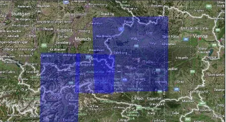
covered parts of Austria which, combined with the availability of appropriate reference data (orthophotos), was the reason for choosing this test site. In addition, the interest lies in the knowledge over Austria, which has high mountains and thus the process of orthorectification can be more difficult (due to errors in a digital terrain model). Sentinel-2 products used in this experiment differ in the size of area covered since they were created out of different number of tiles (one, two and four). Figure 1 shows Sentenel-2 data coverage of Austria during its commissioning phase.
Figure 1. Sentenel-2 data coverage of Austria
Reference data which Sentinel-2 data of Austria was compared to is Geoland Basemap Orthophoto of Austria (data source: LandTirol - data.tirol.gv.at). It is a color image acquired with a photogrammetric camera. The reference data was chosen this way and not vice versa because Geoland Basemap Orthophoto has ground sample distance (GSD) of 20 cm and thus better resolution than the Sentinel-2 orthophoto. Also, its orthorectification was performed using more accurate digital terrain model (the 10 m terrain model of Austria based on airborne laser scanning for Geoland Basemap Orthophoto as opposed to PlanetDEM based on the Shuttle Radar Topography Mission – SRTM for Sentinel-2 orthophoto). The accuracy of Geoland Basemap Orthophoto is better than 1 m.
3.2 Serbia
The second test field was Serbia. This test site was additionally included in the experminet in order to get a better insight in the geometric quality of the Sentinel-2 data. The same methodology (same enitity types, processing steps, etc.) was applied both for Serbian and Austrian test site. At the time when this area was analyzed, a number of Sentinel-2 products covering parts of Serbia were available. Unfortunately, majority of them was useless since clouds covered more than 80% of the observed territory. Nevertheless, some entities convenient for the future analysis could have been detected.
Reference data was represented as orthophoto with GSD of 40 cm and the accuracy of 0.8 m. Its orthorectification was performed with the 25 m digital terrain model of Serbia with the average height accuracy of 1.6 m. The appropriate reference data was delivered by the company Mapsoft, Belgrade, Serbia.
4. EXPERIMENT DESCRIPTION
The first visual comparison of Sentinel-2 data covering Austria with Geoland Basemap Orthophoto of Austria showed that corresponding details in two images are shifted for several pixels. Because of that a statistical parameter was needed to describe this relation. Available reference data source like The International Archives of the Photogrammetry, Remote Sensing and Spatial Information Sciences, Volume XLI-B1, 2016
orthophoto is a standard, with known accuracy, and that is why it was used in this experiment. Out of the possible set of features to compare (point features, texture lines, shadow lines, objects) it was chosen to compare line segments, because visual analysis suggested that scale differences matter least for these features. In other words, visual comparison revealed that finding suitable corresponding points is difficult due to scale difference, whereas it is quite obvious for long linear structures. In the case of choosing appropriate line segments the degree of automation can be high thanks to the algorithms for automatic edge detection and very good initial georeferencing. Thus, many observations can be made in order to have a good base for the statistical evaluation of the geometric quality of Sentinel-2 data. The initial idea was to use airstrips as the most representative entities and ones that can be detected in both images. Having only four airfields in the initial test area covered by the available data, river coasts and roads were additionally included in processing.
The statistical parameter describing the geometrical relation between different images that cover the same area was calculated as a distance di between corresponding curves in two datasets where i=1,2,...,n and n is a number of curves in a sample. These curves were represented by polylines Oi in orthophoto and Si in Sentinel-2 data. The vertices sij (j=1,2,...,mi; mi is a number of vertices in the i-th polyline) of the polyline Si were exported and their absolute distances δij to the corresponding polyline Oi were calculated. The average value di of the distances δij is an estimate of the distance between the two curves. The estimate of the distance between the two datasets d is the average value of all distances di: an entity. Having the whole territory of Austria covered by the orthophoto data, entities to be used in geometry analysis were chosen based on Sentinel-2 data covering only certain parts of Austria. The data was visually inspected first to find some significant entity. After finding such an entity in the Sentinel-2 image, the following step was subsetting the Sentinel-2 data. The reason for this was the big size of the original Sentinel-2 data due to which this data could not be opened afterwards in processing software. Subsetting, together with picking out the appropriate band combination, was done in the official Sentinel-2 toolbox software by defining the extents of the resulting image so that the image includes the chosen entity. The combination of green, red and infra-red band was chosen in order to have a high contrast while maintaining a representation of objects in the images close to those of aerial images.
Then the identical views of the orthophoto and the Sentinel-2 Level 1C image were selected and exported. This eased completing further tasks. A new image was exported with respect to a zoom magnitude and a decision was made to use a resolution where one pixel of the new image equaled one pixel of the Sentinel-2 image, i.e. where one pixel of the new image equaled 10 m. Again, this resolution was used for both datasets. The attempts to use an extreme zoom-in or zoom-out led to bad results in edge detection afterwards. In the extreme zoom-out case entities could not be properly distinguished. Opposite to that, in the extreme zoom-in case, edge detection filter detected edges of every single pixel in the Sentinel-2 image instead of an edge of a whole entity.
The extracted images were multi-band images. In order to perform edge detection these images needed to be converted to grayscale. The equation used for this conversion was such that
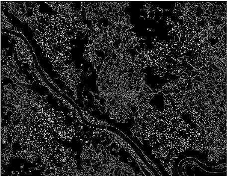
The following step was the edge detection in grayscale images. The same operator was used with all the images to make the processing as homogeneous as possible. Since edges were differently oriented, one direction filters were not a good choice. Sobel and Prewitt filters also did not give good results as they omitted a lot of important parts of edges, so Canny filter was used for the edge detection. It gives an image (raster) like
Figure 2. Edge detection in an orthophoto image; image covers the area of 13 km × 10 km
Since manipulation of edges is much easier when they are represented by vector and not by raster, conversion from raster to vector was performed. Many edges were detected in every single raster image (green lines in Figure 3) and only few lines of interest were needed (red lines in Figure 3), so manual cleanup of redundant edges (green lines which are not included in red lines in Figure 3) was done. As already mentioned, Canny filter does not ideally detect lines. In order to get a valuable polyline which truthfully represented a required edge, a river The International Archives of the Photogrammetry, Remote Sensing and Spatial Information Sciences, Volume XLI-B1, 2016
coast in this case, refinement of detected edges had to be done. Refinement consisted of connecting detected parts of the edge in one polyline, correcting obvious errors in detection of the river coast edge (e.g. a road near the coast was detected instead of the river coast), adding parts of the coast which were not detected at all, etc. This step was the most time consuming. Only at this point can the operator check if the entity chosen at the beginning can easily be detected or it requires a lot of manual correction.
Figure 3. Detected edges in vector format; the red line is the line of interest
Having the line of interest in the orthophoto extracted, the following step was calculation of the proximity raster for that line. In Figure 4 an example of a proximity raster can be seen. The area around the polyline gets brighter as the distance from the polyline increases. The top right corner which is completely white is more than 5 km away from the closest point of the polyline.
Figure 4. Proximity raster; image covers the area of 8.5 km × 8.5 km
Points (vertices) were exported from the polyline extracted from the Sentinel-2 image and each point got a value assigned from the proximity raster which corresponded to the point location. A value assigned to a point did not include information about the side of the polyline on which the point is. The average of the values assigned to the points (Equation 2) was used as a parameter of mismatch between the two polylines, whereas the statistics calculated using Equation 3 represented the mismatch between the two datasets.
The list of the steps undertaken in the experiment among which some could have been avoided if certain preconditions had been met is as follows:
1. Identification of an entity, 2. Subsetting a Sentinel-2 image,
3. Extraction of both Sentinel-2 and orthophoto images, 4. Conversion to grayscale,
5. Edge detection using an appropriate filter, 6. Vectorization,
7. Cleanup and refinement,
8. Rasterization of an orthophoto polyline, 9. Proximity calculation,
10. Extraction of points from a Sentinel-2 polyline, 11. Adding distance values to the points,
12. Distribution of the distance values and calculation of the average distance value.
6. RESULTS AND DISCUSSION
By calculating the statistics, it was shown that the average mismatch between the datasets over the area of Austria is a bit more than 6 m, or about half the size of a Sentinel-2 image pixel, with a standard deviation of about 5 m. The differences between corresponding lines of the orthorectified satellite and aerial images are in the same order of magnitude, with one exception. The example no. 14 showed bigger differences between the polylines and manual check revealed that there were differences in the edge detection around some peninsula (Figure 5). The influence of potential outliers on the final results had to be estimated.
Figure 5. Edge detection differences - a peninsula case
A hypothesis was set to say that outliers have a great impact on the results.
The mean (average; x̅) and the standard deviation (σ) had already been calculated, but since mean is not a robust statistic measure which can be applied to distributions including outliers, the median (x̃) and the robust estimator for the standard deviation of a distribution based on the median of the absolute differences to the median (σMAD) were additionally calculated. Both x̃ and σMAD were calculated in order to be able to compare them with the mean and the standard deviation to see if potential outliers have a significant impact on the results. The The International Archives of the Photogrammetry, Remote Sensing and Spatial Information Sciences, Volume XLI-B1, 2016
differences between the mean and the median (Figure 6), as well as the differences between σ and σMAD (Figure 7) are small, so it can be said that potential outliers do not have a big impact on presented statistics, and therefore our hypothesis can be rejected. As far as the peninsula case is concerned, these differences are not describing errors of orthorectification, but either differences in the object appearance (large influence of water level change due to very low embankment inclination) or actual change (mobilization of sediments).
Figure 6. Mean and median histogram for the test site Austria
Figure 7. σ and σ
MAD histogram for the test site Austria
The test field over Serbia revealed the average mismatch between the two datasets of about 12 m which is more than one pixel of a Sentinel-2 image, with a standard deviation of about 8 m. The differences between the mean and the median (Figure 8), as well as the differences between σ and σMAD (Figure 9) are small in this case as well, so the hypothesis set previously can also be rejected for this test site.
Figure 8. Mean and median histogram for the test site Serbia
Figure 9. σ and σMAD histogram for the test site Serbia
7. CONCLUSION
The obtained results show that Sentinel-2 data has very good geometric quality. Although it is not suitable for tasks which require high accuracy (better than 10 m) it is still reliable for use in other applications. Improvements in edge detection algorithms similar to one presented in (Devernay, 1995) can lead to sub-pixel accuracy in edge positioning. Still, the method presented in the paper offers a reliable estimation of the geometric quality of Sentinel-2 data with options for additional improvements.
Sentinel-2 data is very suitable for tasks which include large areas since it covers the whole globe. Clouds could obscure these images and make them difficult to use, but creation of a cloud-free mosaic would be a good solution to this problem. The frequent revisit time of 10 days with only Sentinel-2A in orbit, and 5 days with both Sentinel-2A and Sentinel-2B in orbit, potentially enables successful creation of this cloud-free mosaic.
The additional benefit of Sentinel-2 data is that it is completely free of charge compared with some other satellite data. People can download and process Sentinel-2 data without any fee. If the final results still do not meet required conditions, they can turn to other data without any financial consequences.
In has to be highlighted that in this project Sentinel-2 data was subsetted and additionally saved as new images using a specific software tool. These images were later on used for processing. This additional step was needed because of the encountered problems in the performance of the software used (in its current version).
Furthermore, edges in the experiment were differently oriented and a single edge detection filter with default values was used. This way the simplicity of the experiment has been preserved. If only one direction edges were needed, perhaps the usage of another filter but Canny would give better results and demand less manual work.
For similar purposes to the one presented in this paper, more complex edge detection methods which might have better accuracy could be investigated in the future work. Another task could be the assessment of an error influence of the edge detection technology on the final results when performed on images with different geometric and radiometric characteristics. The International Archives of the Photogrammetry, Remote Sensing and Spatial Information Sciences, Volume XLI-B1, 2016
REFERENCES
Basu, M., 2002. Gaussian-Based Edge-Detection Methods - A Survey. IEEE Transactions on Systems, Man, and Cybernetics - Part C: Applications and Reviews, 32(3), pp. 252-260.
Canny, J., 1986. A Computational Approach to Edge Detection. IEEE Transactions on Pattern Analysis and Machine Intelligence, 8(6), pp. 679-698.
Devernay, F., 1995. A Non-Maxima Suppression Method for Edge Detection with Sub-Pixel Accuracy. Technical Report RR-2724, INRIA, Sophia Antipolis, France.
Dial, G., Bowen, H., Gerlach, F., Grodecki, J. and Oleszczuk, R., 2003. IKONOS satellite, imagery, and products. Remote Sensing of Environment, 88(1-2), pp. 23-36.
European Space Agency (ESA), 2015. Sentinel-2 User Handbook, issue 1, revision 2, 24/07/2015. 64 pp. https://sentinel.esa.int/documents/247904/685211/Sentinel-2_User_Handbook (31 Mar. 2016).
Greenfeld, J., 2001. Evaluating the Accuracy of Digital Orthophoto Quadrangles (DOQ) in the Context of Parcel-Based GIS. Photogrammetric Engineering & Remote Sensing, 67(2), pp. 199-205.
Juneja, M. and Sandhu, P.S., 2009. Performance evaluation of edge detection techniques for images in spatial domain. International Journal of Computer Theory and Engineering, 1(5), pp. 614-621.
Kakarala, R. and Hero, A.O., 1992. On Achievable Accuracy in Edge Localization. IEEE Transactions on Pattern Analysis and Machine Intelligence, 14(7), pp. 777-781.
Maini, R. and Aggarwal, H., 2009. Study and Comparison of Various Image Edge Detection Techniques. International Journal of Image Processing, 3(1), pp. 1-12.
Novák, D. and Baltsavias, E., 2009. Orthoserv - quality assessment for orthorectified and co-registered satellite image products. In: The International Archives of the Photogrammetry, Remote Sensing and Spatial Information Sciences, Hannover, Germany, Vol. XXXVIII-1-4-7/W5, 7 pp.
Sharifi, M., Fathy, M. and Mahmoudi, M.T., 2002. A Classified and Comparative Study of Edge Detection Algorithms. In: Proceedings of the International Conference on Information Technology: Coding and Computing, pp. 117-120.
Ziou, D. and Tabbone, S., 1998. Edge Detection Technique - An Overview. Pattern Recognition and Image Analysis, 8(4), pp. 537-559.