INVESTIGATIONS ON THE POTENTIAL OF CONVOLUTIONAL NEURAL NETWORKS
FOR VEHICLE CLASSIFICATION BASED ON RGB AND LIDAR DATA
R. Niessnera, H. Schillinga, B. Jutzib
a
Fraunhofer Institute of Optronics, System Technologies and Image Exploitation, Gutleuthausstr. 1, 76275 Ettlingen, Germany - (robin.niessner, hendrik.schilling)@iosb.fraunhofer.de
bInstitute of Photogrammetry and Remote Sensing, Karlsruhe Institute of Technology (KIT), Englerstr. 7, Germany
KEY WORDS:CNN, data fusion, airborne laserscanning, orthofoto, vehicle classification
ABSTRACT:
In recent years, there has been a significant improvement in the detection, identification and classification of objects and images using Convolutional Neural Networks. To study the potential of the Convolutional Neural Network, in this paper three approaches are investigated to train classifiers based on Convolutional Neural Networks. These approaches allow Convolutional Neural Networks to be trained on datasets containing only a few hundred training samples, which results in a successful classification. Two of these approaches are based on the concept of transfer learning. In the first approach features, created by a pretrained Convolutional Neural Network, are used for a classification using a support vector machine. In the second approach a pretrained Convolutional Neural Network gets fine-tuned on a different data set. The third approach includes the design and training for flat Convolutional Neural Networks from the scratch. The evaluation of the proposed approaches is based on a data set provided by the IEEE Geoscience and Remote Sensing Society (GRSS) which contains RGB and LiDAR data of an urban area. In this work it is shown that these Convolutional Neural Networks lead to classification results with high accuracy both on RGB and LiDAR data. Features which are derived by RGB data transferred into LiDAR data by transfer learning lead to better results in classification in contrast to RGB data. Using a neural network which contains fewer layers than common neural networks leads to the best classification results. In this framework, it can furthermore be shown that the practical application of LiDAR images results in a better data basis for classification of vehicles than the use of RGB images.
1. INTRODUCTION
Traffic-related data is the key issue for urban monitoring and planning. Therefore the automated analysis of this data to derive a parametrized characterization is essential. Typical parameters of interest start from precise vehicle location, number of vehicles up to traffic density and flow.
For detection, recognition and classification of vehicles the gra-dient between vehicle and background can be helpful because it often shows a strong characteristic. Therefore gradient-based al-gorithms are utilized to determine vehicles in images, e.g. like Histogram of oriented Gradients (Dalal and Triggs, 2005), local binary patterns (Ojala et al., 1994) or SIFT descriptors (Lowe, 1999). Further statistically predominate image pattern within and around the vehicle area can be of interest and characterized by very high-dimensional feature spaces, referred as implicit ap-proaches (Grabner et al., 2008; Kembhavi et al., 2011; Moran-duzzo and Melgani, 2014). In contrary, explicit approaches rely on the image features with typical features of the vehicle shape (Hinz and Stilla, 2006), such as the vehicle edges and their com-binations, possibly enriched by other information. Beside gradi-ents the region-based approaches are promising. These relies on the assumption that at least piecewise color homogeneity of vehi-cles is given. Various approaches are available, like a top-hat al-gorithm (Zheng et al., 2013), an extended region-growing method (Holt et al., 2009), a segmentation by using Otsu’s method (Eikvil et al., 2009), as well as a method based on the detection of re-gions of salient colors in images (Cheng et al., 2012; Leitloff et al., 2010).
To increase the performance and reduce the false alarm rate
addi-tional knowledge can be considered as constrain (Hinz and Stilla, 2006; T¨urmer et al., 2013). However this constrain has an in-fluence on the classification performance, as not all vehicles are parked on or close to roads (like such parked in backyards) and further highly accurate road maps are mandatory.
Combining measurements from different types of sensors for the analysis is a strategy to increase the performance, especially if the derived data is complementary. Therefore radiometric data in form of RGB images and the geometric data measured with a LiDAR sensor can be considered for vehicle classification. For narrowing the search space of vehicle detection geometric data is favorable (T¨urmer et al., 2013). The LiDAR point cloud can be utilized for extracting vehicles and their motion (Yao et al., 2011). Further features can be estimated by LiDAR point cloud for ob-ject classification in general (Jutzi and Gross, 2009; Weinmann et al., 2015). To derive vehicle hypotheses several features can be calculated in this context by using radiometric (optical) and geo-metric (elevation) data for classification. The fusion of the data sources is done by state-of-the-art-classifier and only geometric data is utilized for generating vehicle hypotheses (Schilling et al., 2015).
In this work we study the potential of Convolutional Neural Net-works especially for vehicle classification. Therefore three ap-proaches are investigated to train classifiers based on Convolu-tional Neural Networks. The main contribution of this work is
• CNNs based on RGB and LiDAR data lead to classification results with high accuracy
• features derived by RGB data transferred into LiDAR data by transfer learning lead to better classification results in contrast to RGB data only
• using a neural network with less layers than common neural networks leads to the best classification results
This contribution is organized as follows. In Section 2 an overview on the most relevant components of a convolutional neural net-work is given. The utilized data is described in Section 3. We use three different approaches to train classifiers based on con-volutional neural networks, the related experiments are described in Section 4. The derived results are presented in Section 5 and discussed in Section 6. Finally we conclude and an outlook on future work is given.
2. METHODOLOGY
The presented work is based on convolutional neural networks (CNN), an advanced development of artifical neural networks (ANN) (LeCun et al., 1998). In this section we show the differ-ences and advantages of CNNs compared to ANNs for 2D clas-sification tasks.
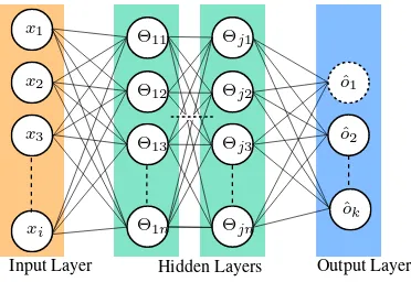
One of the main reasons for the low performance of ANNs in tasks of 2D classification are the fully connected layers (Figure 1). Each input valuexiis connected to all neuronsθ1nand all
neurons from the previous hidden layer are connected to the neu-ronsθjn of the following hidden layer. For a fully connected
ANN with 100 hidden neurons and an input size of80×80 pix-els we need to train 1.92 million weighted connections.
x1
Input Layer Hidden Layers Output Layer
Figure 1. Base concept of a fully connected artificial neural network. The orange layer contains the input information, the
green layers arejhidden layers and the blue output layer consists ofkoutput classes.
The tremendous amount of required training data and computa-tional resources is not the only drawback of fully connected lay-ers for 2D image classification. By giving each neuron all pixels as input the classifier is highly dependent on the object location
in the given image. Furthermore, there is no local correlation be-tween pixels in divergent regions of the image. The image on the left in Figure 2 gives an example for a fully connected convolu-tional layer. Each neuronθnis connected to the complete input
image. The image on the right shows an approach where each neuronθnis connected to a local region of the image called
re-ceptive field. The calculated weight matricesWnfor each neuron
are shared for the whole image. Each neuronθis considered as a filter with the size of the receptive field to compute the convo-lution. Put simply, the filter mask corresponds to the calculated weight matrix which slides over the image. The results aren fea-ture maps wherenis the depth of the following data volume. The convolution (∗) is computed over all channelsiof the input image or the depth of subsequent feature maps:
ˆ
ok=f(
X
i
Win∗xi+bn) (1)
whereWindenotes the weight matrix corresponding to the
chan-neliand neuronn, xi is the input value andbnis a bias. The
outputoˆkis the value which is written in the subsequent feature
map.
Figure 2. On the left a fully connected layer is depicted, each neuron is connected to every value of the input data. On the right
side a locally connected layer is shown, each neuron is connected to a receptive field and the weights of each neuron are
shared for every sampling position of the image.
Using the local connectivity, the classifier becomes translation invariant and the computational cost decreases to a fraction com-pared to the fully connected approach. The required amount of training data also decreases since there are fewer weight parame-ters and biases which need to be computed. But still, the training of deep CNNs requires thousands up to a million of training sam-ples which are usually not given in the field of remote sensing classification tasks.
Figure 3. On the left side a neural network is shown with all neurons activated. On the right side a neural network is depicted
where neurons get deactivated with a probability ofpby a dropout layer to prevent overfitting.
w2
Figure 4. Influence on the convergence of the optimization using the SGD. The figure on the left side shows how the convergence of a 2D optimization should look like for a fitting LR. A LR to
high will lead to a divergence of the optimization as shown in the figure in the middle. In the figure on the right the LR is too low what results into a convergence towards a local minimum.
The outputs have to get adjusted as the deactivated neurons would lead to numerical differences in the outputs between training and test phase. To accomplish this the output values for the test phase get multiplied by the dropout-probabilityp.
Activation Function Another relevant component of CNNs is the activation function between layers. The relu-function is a common activation function in CNNs as they can be computed more efficient than sigmoid or hyperbolic tangent functions and is defined as:
f(x) =max(0, x) (2)
It was shown empirically that the convergence of the stochastic gradient descent (SGD) by (Bottou, 2010) using relu activation functions can be accelerated by a factor of six compared to sig-moid or hyperbolic tangent functions (Krizhevsky et al., 2012a). As activation function of the output classification layer we are using a softmax classifier (Bishop, 2006). The softmax classifier computes the probability of the class affiliation of each input .
Training To understand how a CNN learns the weights we take a glance at three important parts of the CNN. The error between the softmax output and the labels is computed using a cross-entropy loss function (De Boer et al., 2005). To minimize this training error the weights get updated using back-propagation (Hecht-Nielsen et al., 1988). The back-propagation is used to compute error-rates of single neurons to trace back the impact they have on the training error. To compute the updates the data set is divided in mini-batches as the stochastic gradient descent is computing the optimization using only a subset of the data. The most important parameter while training a CNN using SGD is the learning rate (LR). Using a good LR will result in a fast conver-gence of the optimization as shown in Figure 4 (left plot). If the LR is too high the optimization will diverge as shown in Figure 4 (middle). The figure on the right side shows the optimization converging towards a local minimum as the LR is too small.
3. RGB AND LIDAR DATA SET
We use two data sets in this work which were provided by the Im-age Analysis and Data Fusion Technical Committee (IADF TC)
of the IEEE Geoscience and Remote Sensing Society (GRSS) (Moser et al., 2015). The data consists of a RGB and LiDAR data set. Both data sets were acquired using an airborne platform flying over the harbor of Zeebruge, Belgium. The RGB data is a orthophoto with a 5cm ground sampling distance (GSD). The LiDAR Data is provided as a digital surface model (DSM) with a point spacing of 10cm. The LiDAR point cloud gets rastered to a 2D grayscale image by using natural neighbor interpolation. The RGB data is down sampled to 10cm GSD to go with the GSD of the LiDAR data.
Since there is only one data set available we are separating the training and validation data locally to minimize the correlation between the two sets. For training purpose we augment the data by rotating it by 90◦, 180◦and 270◦to create more training sam-ples and make the classifier more robust towards rotation vari-ances. All images also get zero-centered by subtracting the mean value of each channel.
4. EXPERIMENTS
Three different approaches are presented in this work based on CNNs to classify vehicles in RGB and LiDAR. The data sets can be seperated in two fields. In Section 4.1.1 and Section 4.1.2 a pretrained CNN is used, those ideas are based on the concept of transfer learning. In Section 4.2 we design and train a CNN from scratch. Those approaches tackle the requirement of the tremendous amount of training data to train deep CNNs.
4.1 Transfer learning
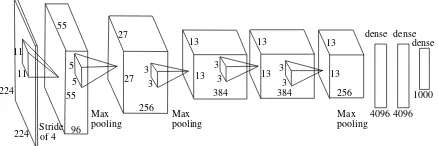
The following two approaches are based on the concept of trans-fer learning. The idea behind those approaches is that CNNs which are trained on one data set can be transferred to classify an other data set. We are using a CNN based on the AlexNet archi-tecture of (Krizhevsky et al., 2012b) depicted in Figure 5 which was pretrained on the ImageNet dataset (Deng et al., 2009).
3
Figure 5. Architecture of the AlexNet, where the most conventional CNN architectures are derived from.
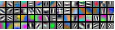
Figure 6. Features of the pretrained VGGNet in the first convolutional layer computed inMATLAB. The appearance of
the filter masks is similar to gabor and blob filters.
4.1.1 CNN Feature Vector In this approach we take away the task of classification from the CNN and we only use it as feature extractor. To accomplish this, we remove the last fully connected layer of the CNN which is usually the classification layer. In this case, the resulting feature map of the convolution of the penulti-mate layer is a feature vector (Nogueira et al., 2016). The size of the feature vector depends on the CNNs architecture, the size is 4096×1. The extracted features are used to train a linear support
feature maps feature vector
4096×1
Figure 7. Changes in the VGGNet to use the output of the last layer as feature vector. The Classification layer is removed and the penultimate layer with the size of4096×1is used as feature
vector.
vector machine (SVM) (Burges, 1998). To fuse the RGB, LiDAR elevation and intensity data we concatenate the feature vectors for the SVM training so the dimensions of the resulting vectors are 4096×1,8192×1and12288×1.
4.1.2 Fine-Tuning In this approach we use the pretrained CNN as feature extractor and classifier. The process of training a pre-trained CNN on a different dataset is called fine-tuning (Nogueira et al., 2016). Again, we have to take a few small adjustments at the CNN. Theoretically, there are no restrictions how many changes can be applied to the architecture of the CNN. Consider-ing there is only a small amount of trainConsider-ing samples available we want to keep the number of parameters we have to retrain as small as possible. Since the VGGNet is trained on the ImageNet data set its classification output layer consists of 1000 elements for the 1000 classes of the ImageNet. As we only want to separate the background and vehicle class we have to change the classification layer to a two element layer. The green highlighted elements in Figure 8 are the ones that replace the old classification layer. The new weights between the penultimate fully connected layer and the classification layer need to be trained since they get initial-ized at random. The rest of the CNN remains the same before the fine-tuning starts.
We kept the learning rate for all layers the same since our ex-periments showed there is no difference in the training outcome regarding the error rate whether we set the learning rate of the pretrained layers to zero or the same as the new layer. The reason for this is how the weights of the layers are changed in the training
feature maps feature vector
4096×1
Figure 8. Changes for fine-tuning the VGGNet on the classification task. The classification layer and the corresponding
weights get replaced by a two element classification layer with weight matrices of the corresponding size.
process of the CNN. An error value for each neuron in the net-work is calculated starting from the output. The backpropagation uses this error value to determine which neuron has the highest impact on the classification error and updates the weights to min-imize this classification error. Since all layers besides the clas-sification layer are already roughly adapted to the clasclas-sification problem the CNN will update the randomly initialized weights of the new classification layer to minimize the classification error.
A disadvantage of this approach is that we can not change the dimensionality of the input data since we do not want to change the pretrained weights in the first layer of the CNN. The number of channels of the input image is limited to the size of the data the CNN was originally trained with. The number of input channels is limited to three, as the VGGNet we are using was trained on a RGB data set. This implies that we can not fuse RGB and LiDAR data at the input layer of the CNN. As there is only one channel available using the LiDAR data sets we simply put that channels information in all three input channels of the VGGNet.
4.2 Training and design from the scratch
This approach is based on designing and training a CNN from scratch. Most state of the art CNNs consist of millions of param-eters and require an huge amount of training samples. As we are training a CNN for a binary classification problem, CNNs with few parameters can probably also solve this problem. It is not necessary to use CNN architectures with that many parameters. In Table 1 the architectures of two best performing CNNs in this study are listed. S is the stride andP the padding of the con-volutional layers. As pooling method we use max-pooling and while training a dropout is used at the first fully connected layer to prevent overfitting. The designed shallow CNNs consisting of only a fraction of parameters compared to deep CNNs such as AlexNet . The size of the filter in the first layer of the Medium-CNN was chosen at a equal dimension as the size of the filter from the AlexNet architecture. The size of the filters of the Large-CNN was chosen to be at the scale of the objects in the image we are going to classify. In contrast to the approach from Section 4.1.2 we can fuse the RGB, LiDAR elevation and intensity data in the input layer of the map. Every combination and number of chan-nels can be chosen since all weights are trained anew every time you change the CNN. The following layers of the CNN are not af-fected by changes of the input layers size since they only depend on the number of neurons in the previous layer.
4.3 HoG feature classification
Medium-CNN Large-CNN
Table 1. Architecture of CNNs designed and trained from the scratch.
the work of (T¨urmer, 2014). The work shows the applicability of the well-known histograms of oriented gradients (HOG) by (Dalal and Triggs, 2005) as input to a state-of-the-art classifier. Following this approach, we extract HOG features at the cen-ter of each segment in RGB, elevation and intensity data sepa-rately, concatenate these features in a single vector and use ran-dom forests for classification (Breiman, 2001). The used segmen-tation algorithm is presented in (Schilling and Bulatov, 2016) As HOG features are sensitive to orientation, we augment the train-ing data through rotation. All relevant parameters (e.g. blocksize and cellsize) as well as sensor combinations are optimized using cross validation.
5. RESULTS
The training of the CNNs was performed on a balanced data set with 399 training samples of each background and car class be-fore data augmentation. As there is way more background than cars in a realistic scenario we use 426 car and 6017 background samples for the validation of the training which were acquired with a watershed based segmentation method (Schilling and Bu-latov, 2016). Since the validation is highly unbalanced the overall accuracy is not fit for representing the quality of the classifica-tion. The F-score, the harmonic mean of precision and recall, is more suitable for this task. The training results are then compared to the classification approach based on the histogram of oriented gradients (HOG) features and a random forest classification.
5.1 Training Results
The training is conducted by utilizing theMatConvNet frame-work inMATLAB(Vedaldi and Lenc, 2015). For the classification layer we use a softmax classifier with a cross-entropy loss func-tion to update the weights. As optimizafunc-tion funcfunc-tion we choose the SGD. The CNN training is applied with LR of0.01,0.001 and0.0001. The training is terminated if the validation loss does not decrease overktraining epochs wherekis defined as
k= 10 +lnumEpoch 10
m
×2. (3)
The following samples of the CNN training only show the best performing combinations of LR and data types.
5.1.1 CNN Feature Vector The training of the SVM with the CNN features is performed by using a 10-fold crossvalidation. The SVM with the lowest loss is used to classify the validation data. As shown in Figure 9 the training on the RGB data achieves the lowest F-Score (0.794) even though the CNN features are originally trained on a RGB data set. The best training result is achieved by the fusion of the elevation and the intensity data set (F-Score =0.929). Adding the RGB data to the fusion of the LiDAR data set still outperforms the solitude training results and yields good results but does not improve the training results of the fusion of the LiDAR data.
0.8
Figure 9.F-Scoresfor the CNN feature training using a SVM.
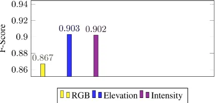
5.1.2 Fine-Tuning For the Fine-Tuning we are using the same pretrained CNN (VGGNet) as we already used in the CNN fea-ture vector approach. For this approach we only get training re-sults for each of the data types, not the fused data. As shown in Figure 10 the training on the LiDAR elevation (F-Score: 0.903) and intensity (F-Score: 0.902) outperforms the RGB (F-Score: 0.867) data training results again. Compared to the results from Figure 9 the training on the solitude data shows improved results for all the data sets.
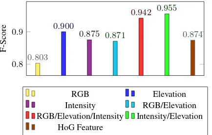
5.1.3 Training and design from scratch For the CNNs de-signed and trained from scratch we take a look at the Medium-CNN and the Large-Medium-CNN. While testing several architectures of CNNs these show the best performance both in computability and training results. As depicted in Figure 11 and Figure 12 the train-ing ustrain-ing the Medium-CNN architecture on the RGB data set (F-Score: 0.803, yellow line with triangles) still under perform the results which are achieved by the training on the LiDAR data. The best training result is achieved by the CNN data fusion of elevation and intensity (F-Score: 0.955, green line with dots). We also compare the result of the Medium-CNN training with a HoG-feature classification using a random forest classifier (F-Score: 0.874, brown line with squares) trained on the fusion of
the RGB and LiDAR data sets. While this classification approach outperforms the results of Medium-CNN on the RGB data, its within the same range as the Medium-CNN trained on the in-tensity data set and the fusion of RGB and elevation data. For the solitude elevation data, the fused data of the LiDAR and the fused RGB and LiDAR data sets the Medium-CNN outperforms the HoG-Feature classification by far.
0.8 0.9
0.803
0.900
0.875 0.871
0.942 0.955
0.874
F-Score
RGB Elevation
Intensity RGB/Elevation RGB/Elevation/Intensity Intensity/Elevation
HoG Feature
Figure 11.F-Scoresfor the training results derived by different data of the Medium-CNN with the HoG feature classification
result for comparison.
0.5 0.6 0.7 0.8 0.9 1
0.5
0.6
0.7
0.8
0.9
1
recall
precision
RGB Elevation Intensity Elevation/Intensity RGB/Elevation/Intensity HoG Feature
Figure 12. PR-Curves of the training results derived by different data for the Medium-CNN with the HoG feature classification
result for comparison.
Figure 13 shows the training results of the Large-CNN. As shown in Figure 13 the training on the RGB data set achieves the low-est F-Score of0.722for all data set combinations. For the CNN-Large the fusion of intensity and elevation produces the best train-ing results with an F-Score of0.927. The HoG feature classifica-tion results lie within the same range as the results for the solitude LiDAR data.
5.2 Sliding window classification
Finally, we want to show a practical result of the CNN based classification approach on our given data set, to see where the weaknesses of the classifier lie and how to tackle or explain them. We chose the Medium-CNN for a sliding window classification on the fusion of LiDAR data as it shows the best performance
0.7 0.8 0.9
0.722
0.878 0.872
0.805 0.845
0.927 0.874
F-Score
RGB Elevation
Intensity RGB/Elevation RGB/Elevation/Intensity Intensity/Elevation
HoG Feature
Figure 13.F-Scoresfor the training results derived by different data of the Large-CNN.
in the training. The classification is performed using a sliding window with a size of80×80pixels. The sampling rate is set to 10 pixel so we can ensure that each car is included and the number of image samples to compute is minimized. For an test area of the size5000×5000pixels we are computing 243049 image samples. In Figure 14 we show samples from the classi-fied area. For visualization purpose we use the RGB image as background even though the data was classified on the fusion of LiDAR data. The classification results are depicted by using a heatmap where the values are interpolated between the classifica-tion values of each classified pixel. On a wide open field where the cars are spread out the classifier has no problems detecting all the cars with almost no false positives. A more challenging task
Figure 14. Samples from the complete classified area. While the classification of the vehicles is performed on the fusion of LiDAR data the results are displayed using the RGB data as background. The heatmap overlay uses the classification values
provided by the Medium-CNN.
is the classification of cars parked close to each other or which are placed in backyard. The left side of Figure 15 shows an ex-ample where a couple of cars are parked next to each other, with a few exceptions the classifier can still separate the cars. The im-age on the right shows an interesting case since the cars are of completely different sizes. The classifier can detect small cars up to large caravans even though the number of training samples for caravans is very low.
Figure 15. Classification samples of different sizes cars off the road. The left image shows cars parked closely together in a parking lot. The classifier is still able to classify them as single
object. In the image on the right side, a classification example for two cars of completely different sizes is shown. Both, the
small car and the caravan are classified as car.
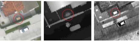
correctly classify the car.
Figure 16. Misclassification of a car covered by a tree. The left image shows the car in the RGB data. In the elevation image in the middle the car is barely visible. In the intensity image on the
right the front of the car is mostly covered by the tree.
Other obstacles are objects which are very similar to cars in their geometry. The image on the left in Figure 17 shows garden furni-ture which looks quite different to a car in the RGB presentation. Looking at the elevation (middle) and intensity (left) representa-tion, the furniture is similar to a small car or the roof of a car. The detector needs to be sensitive for different sizes since the goal is to detect everything from a small car up to a caravan.
Figure 17. Misclassification of an object similar to a car. The left RGB image shows garden furniture which was falsely classified as a car. In the elevation image in the middle and the
intensity image on the right the furniture has the same type of edges like a car roof which may have led to the misclassification.
6. DISCUSSION
In Table 2 we give an overview of all achieved classification re-sults. The best results were achieved by the Medium-CNN de-signed and trained from the scratch on the fusion of the LiDAR data, closely followed by the fusion of RGB and LiDAR data sets. For all proposed approaches the quality of the classification result could be improved by the fusion of the sensor data com-pared to using the solitude data. The only exception is the fusion of RGB and elevation data for the CNNs designed and trained from scratch. The fine-tuning approach could achieve the best training results for the solitude RGB and LiDAR data. Looking
at the overall performance, the LiDAR based classification yield better results than the RGB based classification. This was quite
Data CNN
Feature
Fine-Tuning
From the Scratch
RGB 0.794 0.867 0.803
Elevation 0.846 0.903 0.900
Intensity 0.846 0.902 0.875
RGB/Elevation 0.918 — 0.871
Elevation/Intensity 0.929 — 0.955
RGB/Elevation/Intensity 0.917 — 0.942
Table 2. Overview of the reached F-Scores for all trainings for each data type and combination.
surprising as the CNNs used for the transfer learning approaches (CNN Feature, Fine-Tuning) were pretrained on a RGB data set. This leads to the conclusion that features learned on RGB data are transferable into LiDAR data. The LiDAR data seems to be more suitable for this classification. As we only have a few hun-dred training samples available the uniformity in the geometry of the cars might lead to more stable geometric features than the radiometry from the RGB data as cars of different colors have mostly the same appearance in the LiDAR data. A reason for the decreasing performance by adding the RGB data to the fusion of the LiDAR data might be an imprecise coregistration of the 3D LiDAR data on the 2D RGB data. This leads to blurred edges and as the filters in the first layer of the CNNs are mostly edge detectors. Further, the performance of the Medium-CNN with only 180.000 parameters shows that deep CNNs are not neces-sary for binary classification tasks in this remote sensing applica-tion. The training of the classifiers we present in this work could be performed with only a fraction of training samples compared to common databases for CNN training (e.g. ImageNet).
7. CONCLUSION AND FUTURE WORK
In this paper, three approaches have been presented to classify vehicles from RGB and LiDAR data sets. The novelty of the most successful approach lies in the training of CNNs based on the fusion of RGB and LiDAR data for remote sensing appli-cations. A comparison for different data fusion training results is presented. The CNN with the best performance in training is used for a sliding window classification on the fusion of the elevation and intensity data. We managed to achieve promising training and classification results even though there were only a few hun-dred training samples available. This tackles one of the biggest issues of using CNNs for remote sensing applications. Overall, the training and classification results using the LiDAR data sets outperform the training on the RGB data.
For future work, we want to test more CNN architectures such as siamese CNNs to tackle the problem of a imprecise coregistration and pay more attention to the features of each input channel. An-other field to be examined is the distinction between vehicles of different kinds. Moreover, we intend to test CNN classifications for hyperspectral data and combinations of RGB, hyperspectral and LiDAR data sets.
REFERENCES
Bottou, L., 2010. Large-scale machine learning with stochastic gradient descent. In:Proceedings of COMPSTAT’2010, Springer, pp. 177–186.
Breiman, L., 2001. Random forests. Machine learning45(1), pp. 5–32.
Burges, C. J., 1998. A tutorial on support vector machines for pattern recognition.Data mining and knowledge discovery2(2), pp. 121–167.
Chen, X., Xiang, S., Liu, C. L. and Pan, C. H., 2014. Vehicle detection in satellite images by hybrid deep convolutional neural networks.IEEE Geoscience and Remote Sensing Letters11(10), pp. 1797–1801.
Cheng, H.-Y., Weng, C.-C. and Chen, Y.-Y., 2012. Vehicle de-tection in aerial surveillance using dynamic bayesian networks. IEEE transactions on image processing21(4), pp. 2152–2159.
Dalal, N. and Triggs, B., 2005. Histograms of oriented gradients for human detection. In: 2005 IEEE Computer Society Confer-ence on Computer Vision and Pattern Recognition (CVPR’05), Vol. 1, IEEE, pp. 886–893.
De Boer, P.-T., Kroese, D. P., Mannor, S. and Rubinstein, R. Y., 2005. A tutorial on the cross-entropy method. Annals of opera-tions research134(1), pp. 19–67.
Deng, J., Dong, W., Socher, R., Li, L.-J., Li, K. and Fei-Fei, L., 2009. Imagenet: A large-scale hierarchical image database. In:Computer Vision and Pattern Recognition, 2009. CVPR 2009. IEEE Conference on, IEEE, pp. 248–255.
Eikvil, L., Aurdal, L. and Koren, H., 2009. Classification-based vehicle detection in high-resolution satellite images.ISPRS Jour-nal of Photogrammetry and Remote Sensing64(1), pp. 65–72.
Grabner, H., Nguyen, T. T., Gruber, B. and Bischof, H., 2008. On-line boosting-based car detection from aerial images. ISPRS Journal of Photogrammetry and Remote Sensing63(3), pp. 382– 396.
Hecht-Nielsen, R. et al., 1988. Theory of the backpropagation neural network.Neural Networks1(Supplement-1), pp. 445–448.
Hinz, S. and Stilla, U., 2006. Car detection in aerial thermal im-ages by local and global evidence accumulation. Pattern Recog-nition Letters27(4), pp. 308–315.
Holt, A. C., Seto, E. Y., Rivard, T. and Gong, P., 2009. Object-based detection and classification of vehicles from high-resolution aerial photography. Photogrammetric Engineering & Remote Sensing75(7), pp. 871–880.
Jutzi, B. and Gross, H., 2009. Nearest neighbour classification on laser point clouds to gain object structures from buildings. The International Archives of the Photogrammetry, Remote Sensing and Spatial Information Sciences38(Part 1), pp. 4–7.
Kembhavi, A., Harwood, D. and Davis, L. S., 2011. Vehicle de-tection using partial least squares.Pattern Analysis and Machine Intelligence, IEEE Transactions on33(6), pp. 1250–1265.
Krizhevsky, A., Sutskever, I. and Hinton, G. E., 2012a. Ima-genet classification with deep convolutional neural networks. In: F. Pereira, C. J. C. Burges, L. Bottou and K. Q. Weinberger (eds), Advances in Neural Information Processing Systems 25, Curran Associates, Inc., pp. 1097–1105.
Krizhevsky, A., Sutskever, I. and Hinton, G. E., 2012b. Imagenet classification with deep convolutional neural networks. In: Ad-vances in neural information processing systems, pp. 1097–1105.
LeCun, Y., Bottou, L., Bengio, Y. and Haffner, P., 1998. Gradient-based learning applied to document recognition. Proceedings of the IEEE86(11), pp. 2278–2324.
Leitloff, J., Hinz, S. and Stilla, U., 2010. Vehicle detection in very high resolution satellite images of city areas. Geoscience and Remote Sensing, IEEE Transactions on48(7), pp. 2795–2806.
Lowe, D. G., 1999. Object recognition from local scale-invariant features. In:Computer Vision, 1999. The Proceedings of the Sev-enth IEEE International Conference on, Vol. 2, pp. 1150–1157 vol.2.
Moranduzzo, T. and Melgani, F., 2014. Automatic car counting method for unmanned aerial vehicle images. IEEE Transactions on Geoscience and Remote Sensing52(3), pp. 1635–1647.
Moser, G., Tuia, D. and Shimoni, M., 2015. 2015 ieee grss data fusion contest: Extremely high resolution lidar and optical data [technical committees]. IEEE Geoscience and Remote Sensing Magazine3(1), pp. 40–41.
Nogueira, K., Penatti, O. A. B. and dos Santos, J. A., 2016. To-wards better exploiting convolutional neural networks for remote sensing scene classification.CoRR.
Ojala, T., Pietikainen, M. and Harwood, D., 1994. Performance evaluation of texture measures with classification based on kull-back discrimination of distributions. In: Pattern Recognition, 1994. Vol. 1 - Conference A: Computer Vision amp; Image Pro-cessing., Proceedings of the 12th IAPR International Conference on, Vol. 1, pp. 582–585 vol.1.
Schilling, H. and Bulatov, D., 2016. Segmentation methods for detection of stationary vehicles in combined elevation and opti-cal data. In: International Conference on Pattern Recognition (ICPR), International Society for Optics and Photonics, pp. 592– 597.
Schilling, H., Bulatov, D. and Middelmann, W., 2015. Object-based detection of vehicles in airborne data. In: SPIE Re-mote Sensing, International Society for Optics and Photonics, pp. 9643–420U.
Simonyan, K. and Zisserman, A., 2014. Very deep convolutional networks for large-scale image recognition.CoRR.
Srivastava, N., Hinton, G. E., Krizhevsky, A., Sutskever, I. and Salakhutdinov, R., 2014. Dropout: a simple way to prevent neu-ral networks from overfitting. Journal of Machine Learning Re-search15(1), pp. 1929–1958.
T¨urmer, S., 2014. Car detection in low frame-rate aerial imagery of dense urban areas. PhD thesis, TU M¨unchen, Institut f¨ur Pho-togrammetrie und Kartographie.
T¨urmer, S., Kurz, F., Reinartz, P. and Stilla, U., 2013. Airborne vehicle detection in dense urban areas using hog features and dis-parity maps. Selected Topics in Applied Earth Observations and Remote Sensing, IEEE Journal of6(6), pp. 2327–2337.
Vedaldi, A. and Lenc, K., 2015. Matconvnet: Convolutional neu-ral networks for matlab. In:Proceedings of the 23rd ACM inter-national conference on Multimedia, ACM, pp. 689–692.
Weinmann, M., Schmidt, A., Mallet, C., Hinz, S., Rottensteiner, F. and Jutzi, B., 2015. Contextual classification of point cloud data by exploiting individual 3d neigbourhoods. ISPRS Annals of the Photogrammetry, Remote Sensing and Spatial Information Sciences2(3), pp. 271.