SPECTRAL FEATURE ANALYSIS FOR QUANTITATIVE ESTIMATION OF
CYA-NOBACTERIA CHLOROPHYLL-A
Yi Lin a,b, Zhanglin Ye a,b, Yugan Zhang a,b, Jie Yu a,b
a College of Surveying and Geoinformatics, Tongji University, Shanghai 200092, China-(linyi, 2011_jieyu)@tongji.edu.cn,[email protected],[email protected]
b Research Center of Remote Sensing and Spatial Information Technology, Tongji University, Shanghai 200092, China-(linyi,
2011_jieyu)@tongji.edu.cn,[email protected],[email protected]
KEY WORDS: Chlorophyll-a, Spectral analysis, Multivariate statistical analysis, Vegetation indices, Broad band, Narrow band
ABSTRACT:
In recent years, lake eutrophication caused a large of Cyanobacteria bloom which not only brought serious ecological disaster but also restricted the sustainable development of regional economy in our country. Chlorophyll-a is a very important environmental factor to monitor water quality, especially for lake eutrophication. Remote sensed technique has been widely utilized in estimating the concentration of chlorophyll-a by different kind of vegetation indices and monitoring its distribution in lakes, rivers or along coastline. For each vegetation index, its quantitative estimation accuracy for different satellite data might change since there might be a discrepancy of spectral resolution and channel center between different satellites. The purpose of this paper is to analyze the spec-tral feature of chlorophyll-a with hyperspectral data (totally 651 bands) and use the result to choose the optimal band combination for different satellites. The analysis method developed here in this study could be useful to recognize and monitor cyanobacteria bloom automatically and accurately.
In our experiment, the reflectance (from 350nm to1000nm) of wild cyanobacteria in different consistency (from 0 to 1362.11ug/L) and the corresponding chlorophyll-a concentration were measured simultaneously. Two kinds of hyperspectral vegetation indices were applied in this study: simple ratio (SR) and narrow band normalized difference vegetation index (NDVI), both of which consists of any two bands in the entire 651 narrow bands. Then multivariate statistical analysis was used to construct the linear, power and exponential models. After analyzing the correlation between chlorophyll-a and single band reflectance, SR, NDVI respectively, the optimal spectral index for quantitative estimation of cyanobacteria chlorophyll-a, as well as corresponding central wavelength and band width were extracted. Results show that: Under the condition of water disturbance, SR and NDVI are both suitable for quantita-tive estimation of chlorophyll-a, and more effective than the traditional single band model; the best regression models for SR, NDVI with chlorophyll-a are linear and power, respectively. Under the condition without water disturbance, the single band model works the best. For the SR index, there are two optimal band combinations, which is comprised of infrared (700nm-900nm) and blue-green range (450nm-550nm), infrared and red range (600nm-650nm) respectively, with band width between 45nm to 125nm. For NDVI, the optimal band combination includes the range from 750nm to 900nm and from 700nm to 750nm, with band width less than 30nm.For single band model, band center located between 733nm-935nm, and its width mustn’t exceed the interval where band ce n-ter located in.
custom-ized sensors for cyanobacteria bloom monitoring at a low altitude. In other words, this study is also the basic research for developing the real-time remote sensing monitoring system with high time and high spatial resolution
1. INTRODUCTION
In recent years, lake eutrophication caused a large of Cyano-bacteria bloom which not only brought serious ecological dis-aster but also restricted the sustainable development of regional economy in our country, it has become a pretty serious envi-ronmental problem. In order to reduce the water pollution caused by cyanobacterial bloom and ensure the safety of drink-ing water, many satellite data have been used to study the spa-tial distribution (Matthew, 2012), and the biomass quantitative retrieval (LIU Tangyou, 2002; Heng Lyu, 2013) for water bloom. Biological risk caused by cyanobacteria bloom was evaluated, while cyanobacteria bloom was monitored and predicted, and water quality early warning system was established (Gower, 1994; Adam, 2000; FENG Jiangfan et al, 2009). These satellite data can be classified into wide band multispectral data and narrow band hyperspectral data according to the spectral resolu-tion, hyperspectral data generally comes from field spectrometer and aerial image. According to the previous researches, narrow band can provide more significant information about the physi-cal characteristics for quantitative research.
Chlorophyll-a is a kind of important environment factor which can be utilized to evaluate water quality, nutrient load and pol-lution level. In the past decades, many vegetation indices were used to quantify the biological variation of aquatic plants, for example Simple Ratio (SR) is often used to estimate the biolog-ical variation, such as cyanobacteria, leucocyan etc. Normalized Difference Vegetation Index (NDVI) is an effective index that can monitor vegetation and ecotope (Ekstran, 1992; MA Rong-hua et al, 2005; Sachidananda Mishra, 2013; Wesley J.Moses, 2012; Changchun Huang, 2014). In spite of the same vegetation indices, there also would be discrepancy in quantitative estima-tion precision, since the band locaestima-tion and width of satellite spectral channel are different. As for spectral index, the center location and band width have a lot of impact on the precision of quantitative estimation.
The main purpose of this paper is to analyze the quantified abil-ity for chlorophyll-a corresponding to different vegetation indi-ces calculated from hyperspectral data. Optimal spectral indiindi-ces
and what band wavelength and band center were determined, which are suitable for quantitative estimation for the chloro-phyll-a of cyanobacteria. So that hyperspectral data redundancy can be reduced and the accuracy can be improved while quanti-tative estimating cyanobacteria. The results significantly pro-vide basic research to monitoring and early warning on cyano-bacteria bloom using multispectral data or hyperspectral data.
2. DATA AND METHOD 2.1 Algae selection
Cyanobacterial blooms are common phenomena which are caused by eutrophication (KONG Fanxiang et al, 2005). Cya-nobacteria could come into bloom when the natural condition becomes suitable for cyanobacteria. Microcystic aeruginosa is the one of the most common cyanobacteria species, which can lead to bloom easily, in China. The majority of previous re-searches usually used the Microcystic aeruginosa, captuered in laboratory, whose feature is different from the wild Microcystic aeruginosa in micromorphologic, macromorphologic and cybotactic state. However, it could rarely gather together and generate bloom. Thus in our experiment the control experiments were conducted by using wild Microcystic aeruginosa in Tai Lake.
2.2 Control experiment
The FieldSpecFR spectrometer manufactured by American ASD Company has been applied in this research. The spectrum con-sist of visible and near-infrared (VNIR), short wave infrared 1 (SWIR1) and short wave infrared 2 (SWIR2). After interpolat-ing the spectral channels, spectral data was obtained, of which the spectral resolution is 1nm. The VNIR range (350nm-1000nm) was used in our research.
(400nm-800nm). The probe of spectrometer was vertically placed over the container, looking straight down at a height of 0.3m from water surface. Surface detection range was a circle with a radius of 0.067m. During the experiment, firstly enough water was poured into the container (water is pure without sus-pended solids). Then a certain amount of Microcystic aerugino-sa was added drop by drop, meanwhile stirred uniformly. Each time after adding Microcystic aeruginosa, three samples were collected to obtain the concentration of chlorophyll-a, and measured spectral data three times (under the condition of water disturbance). Five minutes later, when the water came back calm and Microcystic aeruginosa distributed uniformly on water surface, spectral data was measured three times again (under the condition of water stationary). These two containers were uti-lized alternately during the experiment. Totally, 16 groups of different concentration spectral data were collected. The con-centration of chlorophyll-a increased at the speed of 1.3 times, ranging from 0-1190.46 g/L. To obtain more reference data, in the second experiment, the same procedure was performed. A group of sub-experiments were under the condition of disturb-ance, and the range of chlorophyll-a concentration was 15.31 g/L-450.9 g/L (12 gradients). Then a group of sub-experiment was under the condition of water stationary, the range of chlorophyll-a concentration was 143.64 g/L -1362.11 g/L (9 gradients).
The spectral reflectance is calculated by the following equation:
T
Where
T= spectral reflectance LT=target radiance Lr=reference plate radiance =reference plate reflectanceIn our research, a standard gray plate was used as the reference plate, whose reflectance is 30%. The quantitative estimation ability of narrow band vegetation models, broad band vegeta-tion indices models and chlorophyll-a were compared respec-tively, based on which the optimal spectral width can be ex-tracted. Meanwhile Landsat ETM+ bands were selected as the representative of broad bands. Spectral response function was used, and spectral response values of Landsat ETM+’s first 4 bands were simulated by ASD spectral reflectance (Steven et al,
2003). Before applying convolution to ASD spectral reflectance, smoothing processing was not used while obtaining the broad band spectral data.
2.3 Multivariate statistical analysis
Multivariate statistical analysis is generally applied in the study of ocean color remote sensing (Andrew Clive Banks, 2012). Original spectrum, simple ratio (SR) and normalized difference vegetation index (NDVI) (Table 1) were chosen as independent variables, and the concentration of Microcystic aeruginosa chlorophyll-a was regarded as the dependent variable. Pearson product-moment correlation coefficient (r) was calculated to describe the correlation between dependent variable (y) and independent variable (x):
Where x= average of independent variables y=average of dependent variables
n= the number of dependent variables/independent var-iables
Then intervals in which x, y located with high degree of corre-lation were chosen to construct a linear prediction model.
Actually, there might be non-linear relationship between origi-nal spectrum, SR, NDVI and chlorophyll-a respectively, so another two non-linear prediction models were used: power and exponential in addition:
According to the result of determination coefficient (R2):
tained in the first experiment were applied as forecast samples, then the data from second experiment were regarded as test samples.
3. RESULTS AND ANALYSIS
Spectral reflectance of water and Microcystic aeruginosa with different concentration were obtained by control experiments, under the condition of water disturbance and stationary. Spectral reflectance of bands whose wavelength located between 350nm-1000nm was used. Meanwhile two different narrow band vegetation indices and corresponding broad band vegeta-tion indices were calculated (Table 1). Narrow band vegetavegeta-tion indices consisted of any two bands in the entire 651 narrow bands while broad band vegetation indices were the combina-tions of Landsat ETM+ NIR and RED bands.
These specific spectral indices were:
Broad band ETM SR and NDVI indices;
Narrow SR and NDVI indices: any two bands in the entire 651 bands.
Vegetation indices Definition
SR
Broad band SR NIR
RED
Narrow band SR j
ij i
NDVI
Broad band RED
RED
NIR NDVI
NIR
Narrow band NDVIij j i j i
Table 1: Spectral vegetation indices used in this paper
Where NIR = Landsat ETM+ B4 bands RED = Landsat ETM+ B3 bands.
3.1 Correlation of single band reflectance and Microcystic aeruginosa chlorophyll-a
Figure 1 shows the correlation coefficient (r) between single band reflectance and chlorophyll-a under the condition of water disturbance and stationary.
The trend of r is very close to the Microcystic aeruginosa
spec-tral reflectance. In the band intervals in which r decreased and increased quickly, Microcystic aeruginosa spectral reflectance has the similar change. In this area, reflectance is very sensitive to chlorophyll-a concentration. The location of 3 minimum reflectance is corresponding to 3 reflection troughs of Microcys-tic aeruginosa spectrum; the location of 3 maximum is corre-sponding to Microcystic aeruginosa spectral green range peak, secondary band peak, red edge respectively.
Figure 1 Correlation coefficient between Microcystic aerugino-sa spectral reflectance and chlorophyll-a concentration
3.2 Correlation of broad band vegetation indices and Mi-crocystic aeruginosa chlorophyll-a
Under the condition of water disturbance and stationary, corre-lation coefficient (r>0.9) of Microcystic aeruginosa chloro-phyll-a with band 2, band 4 are both very high. At band 1 and band 3, correlation coefficient (r<0.5) is low under the condition of water disturbance. On the contrary, r is more than 0.85 under the condition of water stationary (Figure 2).
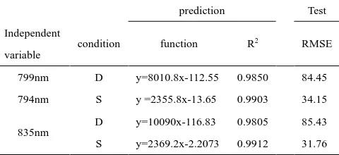
The independent variables include single band reflectance from 733nm to 794nm, ETM’s band 4 reflectance whose central band is 835nm, the SR and NDVI consisted of ETM’s band 3 & 4 and ETM’s band 3 & band 4 central bands. With these variables, linear prediction model of chlorophyll-a was constructed. The precision was evaluated by calculating determination coefficient and RMSE (Table 2).
prediction Test Independent
variable
condition function R2 RMSE
799nm D y=8010.8x-112.55 0.9850 84.45 34.15 85.43 31.76 794nm S y =2355.8x-13.65 0.9903
ETM_B4 D y=9818x-116.6 0.9812 87.23 32.34
30.9
53.82
31.96
53.46 113.8 133.7 111.6 133 S y=2373x-3.518 0.9912
ETM_SR D y=341.4x-233.5 0.9928 S y=124.8x-98.87 0.9921 C_SR
D y=364.19x-241.6 0.9956
S y=127.98x-98.01 0.9921 ETM_NDVI
D y=1276.4x+125.7 0.8693 S y=985.4x-68.04 0.7193 C_NDVI
D y=1293.5x+149.92 0.8776 S y=983.1x-56.508 0.7258
Table 2: linear model
ETM_SR and ETM_NDVI were used to represent broad band indices and C_SR and C_NDVI to narrow band indices. Water disturbance and stationary was abbreviated as D and S respec-tively. The relation between chlorophyll-a real value Y and pre-dicted value y is:
*
ya Y b (4)
Where a= gain b = bias
The RMSE is regarded as a scale used to compare each model’s predictive ability. By comparing RMSE, under the condition of water disturbance, the predictive precision of SR model is high-er, even though the R2 of single band model and SR model are both very high. Hence there is almost little discrepancy between narrow SR model and broad band SR model. Under the condi-tion of water stacondi-tionary, SR model’s predictive precision is low-er than that single band model’s, where RMSE of SR model is 1.7 times higher than that of single band model. The predictive ability of ETM+’s band 4 model is close to which of 794nm model.
3.3 Correlation of narrow band vegetation indices and Mi-crocystic aeruginosa chlorophyll-a
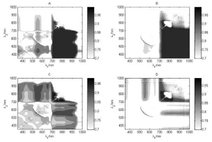
Narrow band SR and NDVI indices consist of any two bands in the entire 651 narrow bands (651*651=423801) were calculated. All narrow band SR and NDVI were chose as independent var-iable and chlorophyll-a is as dependent variable to construct linear regression model. R2 was calculated and shown in Figure 2.The abscissa axis λ1 and vertical axis λ2 are ρj band and ρi band
respectively, which were applied to SR and NDVI indices. The results of SR’s linear regression models under the condition of water disturbance and stationary are shown in Figures 3 (A and B). While the results of NDVI’s linear regression models under the condition of water disturbance and stationary are shown in Figures 3 (C and D).
According to the results above, in each isogram, 6 groups of SR and NDVI indices were extracted where R2 is the biggest, as well as corresponding band center λ1, λ2 and band width ∆λ1, ∆λ2 respectively. The area where R2>0.97 was divided into two parts (R2>0.99 and 0.97<R2<0.99). In the part where R2>0.99, 4 rectangular regions can be extracted. They were SR indices SR1/2/3/6 under condition of water disturbance.
Figure 2 R2’s isogram of narrow band SR, NDVI and chlorophyll-a
Strong linear correlations has been shown between these 6 in-dices and chlorophyll-a. Estimation ability of all SR indices that meet the following equation to chlorophyll-a is similar.
2 2
1 1
ρ
(
λ
±
Δ
)
SR1=
ρ
(
λ
±
Δ
)
ji
(5)
Where Δ1 = 0-Δλ1/2 nm Δ2 = 0-Δλ2/2 nm
condition of water disturbance (Δλ1=362nm, Δλ2=227nm).
3.4 Non-linear correlation of vegetation indices and chloro-phyll-a
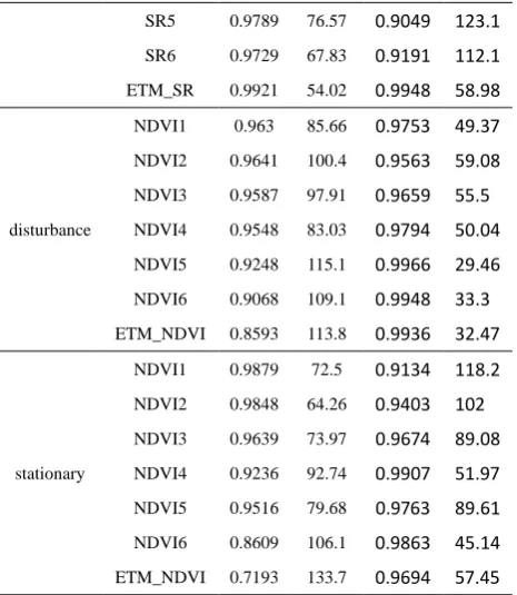
Figure 2 illustrates the linear correlation of SR, NDVI indices and Microcystic aeruginosachlorophyll-a. However, sometimes there may be non-linear correlation between vegetation indices and chlorophyll-a. In our research, power model is the optimal non-linear model. 6 groups of optimal linear models’ band cen-ter (λ1 and λ2) and band width (Δλ1 and Δλ2) were applied to calculate non-linear models. R2 and RMSE (Table 3) were cal-culated by optimal linear models and power models.
As shown in Table 3, for SR indices, SR1/2/3 linear models are better than those power models. While SR4/5/6 power models are better than those linear models under the condition of dis-turbance. Only SR4 power model performed better than those linear models under the condition with disturbance. For NDVI, under the condition of disturbance, estimation precision of power models is superior to their linear models. Under the con-dition of stationary, NDVI 1/2/3/5 linear models performed better than their power models. NDVI 4/6 and ETM_NDVI power models performed better than their linear models.
After comparing SR and NDVI, the indices’ quantitative esti-mation precision of SR 1/2/3/4/6 indices and NDVI 5/6 can perform pretty well under the condition of water disturbance. SR indices and NDVI indices’ quantitative estimation precision to chlorophyll-a are similar, which both performed worse than their single band models.
Linear model Power model condition index R2 RMSE R2 RMSE
disturbance
SR1 0.995 31.76 0.9883 39.24
SR2 0.9971 31.46 0.9899 35.66
SR3 0.9947 36.04 0.9879 36.61
SR4 0.9631 69.44 0.9951 27.89
SR5 0.9582 135.3 0.9171 76.04
SR6 0.9916 44.17 0.9873 36.56
ETM_SR 0.9952 30.9 0.9878 39.52
stationary
SR1 0.9934 47.19 0.9949 49.02
SR2 0.9927 46.55 0.9947 50
SR3 0.9928 47.61 0.9946 52.13
SR4 0.9782 55.33 0.9952 47.88
SR5 0.9789 76.57 0.9049 123.1
SR6 0.9729 67.83 0.9191 112.1
ETM_SR 0.9921 54.02 0.9948 58.98
disturbance
NDVI1 0.963 85.66 0.9753 49.37
NDVI2 0.9641 100.4 0.9563 59.08
NDVI3 0.9587 97.91 0.9659 55.5
NDVI4 0.9548 83.03 0.9794 50.04
NDVI5 0.9248 115.1 0.9966 29.46
NDVI6 0.9068 109.1 0.9948 33.3
ETM_NDVI 0.8593 113.8 0.9936 32.47
stationary
NDVI1 0.9879 72.5 0.9134 118.2
NDVI2 0.9848 64.26 0.9403 102
NDVI3 0.9639 73.97 0.9674 89.08
NDVI4 0.9236 92.74 0.9907 51.97
NDVI5 0.9516 79.68 0.9763 89.61
NDVI6 0.8609 106.1 0.9863 45.14
ETM_NDVI 0.7193 133.7 0.9694 57.45
Table 3: 6 optimal linear models and non-linear models
3.5 Distribution of optimal bands
For the above 6 groups of indices, the optimal 4 groups were chosen to calculate the distribution of corresponding band cen-ter and band width shown in Figure 4 & 5 .
Figure 3: Distribution of SR and NDVI indices’ band center
Figure 4: Distribution of SR and NDVI indices’ band width
band centers of ρi are between 450nm-550nm and 600nm-650nm. And the most optimal band center of ρj (λ1, NIR) locates in the range of 700nm-900nm. The most optimal band widths locate between 46nm-125nm and more than 125nm. For NDVI, most ρi locate in the range from 700nm to 750nm, and most ρj are between 750nm-900nm. Obviously, for SR indices, broad bands take an absolute advantage for quantitative esti-mating Microcystic aeruginosa chlorophyll-a. For NDVI, the narrower bands have, the better quantitative ability is.
4. CONCLUSIONS
By performing two control experiments, the correlation between chlorophyll-a and single band reflectance, SR, NDVI were ana-lyzed respectively. Linear and non-linear regression models were constructed. Then various spectral indices, which were suitable for quantitative estimation of Microcystic aeruginosa chlorophyll-a, their central band wavelength and band width were obtained, which are summarized herewith:
(1) Selecting spectral indices: Under the condition of water disturbance, SR and NDVI indices are both suitable for quantitative estimation of chlorophyll-a, which both performed better than those single band models. Linear model was suitable for SR indices, and power model was suitable for NDVI, under the condition of water stationary, single band models can esti-mate the concentration of chlorophyll-a pretty well, while SR and NDVI indices performed worse.
(2) Selecting band centers and width of spectral indices: For the SR index, there are two optimal band combinations, which is comprised of infrared (700nm-900nm) and blue-green range(450nm-550nm), infrared and red range (600nm-650nm) respectively, with band width between 45nm to 125nm. For NDVI, the optimal band combination includes the range from 750nm to 900nm and from 700nm to 750nm, with band width less than 30nm.For single band model, band center located be-tween 733nm-λ35nm, and its width mustn’t exceed the interval where band center located in.
Our experiments analyzed the quantified ability between Mi-crocystic aeruginosa chlorophyll-a and different vegetation indices under the disturbance and stationary conditions. The following two aspects could be improved: 1) Besides Microcys-tic aeruginosa, there is much suspended matter, chromophoric
dissolved organic matter and so on which can influence the spectrum in lakes; 2) Atmospheric influence was ignored during simulating Landsat ETM data. So our results should be verified in the lake water.
ACKNOWLEDGEMENTS
Data were collected on the roof of Liren Building in FuDan University, we wish to express our gratitude to this. In addition, we wish to give a special thanks to Dr. Mingzhi QU from Queen’s University, who provided much assistance in practices and theoretical guidance.
REFERENCES
FENG Jiangfan, TENG Xuewei, ZHANG Hong, XU Jie. 2006. Forewarning System of Blue Algae for Taihu Lake Based on GIS, 29(9):60-64.
HU Wen, WU Wenyu, KONG Qingxin, XUN Shangpei, WANG Yulan. 2002. Research on Estimating the Concentrations of Chlorophyll-a in Chaohu Lake Using FY-1C/CAVHRR Data, 25(1):124-128.
KONG FanXiang, GAO Guang. 2005. Hypothesis on cyano-bacteria bloom-forming mechanism in large shallow eutrophic lakes, 25(3):589-595.
LIU TangYou, KUANG DingBo, YIN Qiu. 2002. The Spectrum experiments of Algae and Studies On Retrieval Quantitative Information From Its Spectra, 21(3):213-217.
MA Ronghua, KONG Fanxiang, DUAN Hongtao. 2008. Spa-tio-temporal distribution of cyanobacteria blooms based on satellite imageries inLake Taihu, China, 20(6):687-694.
Adams CM, Mulkey D, Hodges A, MilonJW . 2000. Develop-ment of an economic impact assessDevelop-ment methodology for oc-currence of red tide. SP 00-12. Inst Food AgricSci, Food Re-source Econ Dept, Univ Florida, Gainesville, Florida, 58 pp.
Changchun Huang , Jun Zou , Yunmei Li et al. 2014. Assess-ment of NIR-red algorithms for observation of chlorophyll-a in highly turbid inland waters in China. ISPRS Journal of Photo-grammetry and Remote Sensing, 93:29–39.
Vege-tation Indices. Remote Sensing of Environment, 54:38-48.
Daniela Gurlin, Anatoly A. Gitelson, Wesley J.Moses. 2011. Remote estimation of chl-a concentration in turbid productive waters — Return to a simple two-band NIR-red model. Remote Sensing of Environment, 115: 3479– 3490.
Andrew Clive Banks, Pascal Prunet, Julien Chimot et al, A sat-ellite ocean color observation operator system for eutrophica-tion assessment in coastal waters, Journal of Marine Systems, Volume 94, Supplement, June 2012, Pages S2-S15, ISSN 0924-7963.
Ekstrand, S., 1992. Landsat TM based quantification of chloro-phyll-a during algae blooms in coastal. Int. J. Remote Sens. 10, 1913–1926.
Donald C. Rundquist, Luoheng Han, John F. Schalles et al. 1996. Remote Measurement of Algal Chlorophyll in Surface Waters: The Case for the First Derivative of Reflectance Near 690 nm. Photogrammetric Engineering & Remote Sens-ing,62:195-200.
EssayasKabaa, William Philpot, TammoSteenhuis. 2014. Evalu-ating suitability of MODIS-Terraimages for reproducing his-toricsediment concentrations in water bodies: Lake Tana, Ethio-pia. International Journal of Applied Earth Observation and Geoinformation. 26: 286–297.
Gilerson, A.A., Gitelson, A.A., Zhou, J., Gurlin, D., Moses, W.J., Ioannou, I., Ahmed, S.A., 2010. Algorithms for remote estima-tion of chlorophyll-a in coastal and inland waters using red and near-infrared bands. Optics Express 18, 24109-24125.
Giltelson A., Kondratev K. 1991. Peak near 700nm in reflec-tance spectrum of productive waters and its application for re-mote monitoring of water quality. Transactions Doklady of the USSR Academy of Sciences: Earth Science Section,306:1-4.
GOWER, J.F.R., 1994. Red tide monitoring using AVHRR HRPT imagery from a local receiver. Remote Sensing of Envi-ronment, 48, pp. 309–318.
HengLyu, QiaoWang, ChuanqingWuet al.2013. Retrieval of phycocyanin concentration from remote-sensing reflectance using a semi-analytic model in eutrophic lakes. Ecological In-formatics 18 : 178–187.
Matthews, M., Bernard, S., & Robertson, L. 2012. An algorithm
for detecting trophic status (chlorophyll-a), cyanobacteri-al-dominance, surface scums and floating vegetation in inland and coastal waters. Remote Sensing of Environment, 124, 637–652.
Huete A, Didan K, Miura T et al. 2002. Overview of the radio-metric and biophysical performance of the MODIS vegetation indices. Remote Sensing of Environment, 83:195–213.
Luoheng Han and Karen J. Jordan. 2005. Estimating and map-ping chlorophyll-a concentration in Pensacola Bay, Florida us-ing Landsat ETM+ data. International Journal of Remote Sens-ing,26(23):5245-5254.
Wei Shi, Junwu Tang. 2011. Water property monitoring and assessment for China's inland Lake Taihu from MODIS-Aqua measurements. Remote Sensing of Environment 115: 841–854.
Robert K. Vincenta,XiaomingQina,R. Michael L. McKay et al. 2004. Phycocyanin detection from LANDSAT TM data for mapping cyanobacterial blooms in Lake Erie. Remote Sensing of Environment,89:381–392
SachidanandaMishra , Deepak R. Mishra. 2012. Normalized difference chlorophyll index: A novel model for remote estima-tion of chlorophyll-a concentraestima-tion in turbid productive waters. Remote Sensing of Environment, 117:394–406.
Sachidananda Mishra, Deepak R. Mishra, Zhongping Lee et al.2013. Quantifying cyanobacterial phycocyanin concentration in turbid productive waters:A quasi-analytical approach. Re-mote Sensing of Environment, 133:141–151.
Steven, M., Malthus, T., Baret, F., Xu, H., & Chopping, M. 2003. Intercalibration of vegetation indices from different sen-sor systems. Remote Sensing of Environment, 88(4), 412–422.
Y. Chao Rodríguez, A. el Anjoumi, J. A. Domínguez Gómez et al. 2014. Using Landsat image time series to study a small water body in Northern Spain. Environ Monit Assess, 186:3511-3522.