Coarse-grained reverse engineering of genetic regulatory
networks
Mattias Wahde
a,b,*, John Hertz
aaNordita,Blegdams
6ej17,2100Copenhagen,Denmark bDi
6ision of Mechatronics,Chalmers Uni6ersity of Technology,412 96Gothenburg,Sweden
Abstract
We have modeled genetic regulatory networks in the framework of continuous-time recurrent neural networks. A method for determining the parameters of such networks, given expression level time series data, is introduced and evaluated using artificial data. The method is also applied to a set of actual expression data from the development of rat central nervous system. © 2000 Elsevier Science Ireland Ltd. All rights reserved.
Keywords:Genetic regulatory networks; Neural networks; Gene expression
www.elsevier.com/locate/biosystems
1. Introduction
In recent years, the available amount of gene expression data has been increasing at a rapid rate, and there now exist large data sets with expression level measurements from different tis-sue types and different organisms. The existence of time series data, i.e. measurements of the time variation of the expression levels of a number of genes, raises the possibility of determining the regulatory interactions between genes. Recently, there have been many efforts to model genetic regulatory networks and to determine the interac-tions within them, using several different mathe-matical frameworks (see e.g. Kauffman, 1993; Reinitz and Sharp, 1995; Somogyi, 1996;
D’Haeseleer et al., 1999). However, usually the data available are not sufficient to determine ac-curately the interactions between all the genes in a given data set. Therefore it is essential to be able to construct a coarse-grained description of the system, using suitable macroscopic variables. Here we employ the approach of Wen et al. (1998), who clustered the genes into a small number of groups according to their temporal expression patterns, but our method can also be applied to other coarse-graining schemes.
In this contribution we model regulatory works as continuous-time recurrent neural net-works. Our model is introduced in Section 2, and the method is described in Section 3. In Sections 4 and 5, we present the results of applying our method to artificial and real data, respectively. Our conclusions, together with some directions for further work, are given in Section 6.
* Corresponding author.
E-mail address:[email protected] (M. Wahde)
2. The model
We have chosen to model genetic networks using a set of coupled non-linear differential equa-tions. The use of continuous-valued functions en-abled us to model the dynamics at intermediate expression levels, rather than only at the extreme on (1) and off (0) levels. Also, the use of differen-tial equations rather than difference equations allowed us to introduce explicit rate constants. Specifically, we have modeled the networks by equations corresponding to continuous-time re-current neural networks (see Reinitz and Sharp, 1995)
−1are rate constants,x
iare the expression levels, and x;i are their derivatives with respect to time. For a set of N genes, there are N×N
weights (wij), Nbias terms (bi), and N time con-stantsti, i.e. a total ofN(N+2) parameters to be
determined. In principle, one could go beyond the linear additive summation in Eq. (1), and include higher order terms in a network of the form
tix;i+xi=g
bi+%Such terms can implement the complex computa-tional logic carried out by actual regulatory ele-ments (see Yuh et al., 1998). However, the determination of the parameters of a network incorporating higher-order terms would require much more data than is generally available for these systems. Thus, we have limited ourselves to models of the form in Eq. (1).
The non-linear activation function g can be chosen in several different ways. We have chosen to use the logistic sigmoid
g(z)= 1
1+e−kz (3)
Of course one could have used other sigmoid forms as well (e.g. arctan, as used in Reinitz and Sharp, 1995), but at the level of the present analy-sis, there would be no qualitative difference in the results. The choice of the numerical value of k is not very important, since the weights and bias
terms always can be resealed to give the same dynamics for different values of k. We have used
k=1.
3. Method for reverse engineering
There are a number of methods available for determining the weights of a network described by Eq. (1), such as, for example, gradient descent methods (e.g. backpropagation), and simulated annealing. In this investigation, we have chosen to use a genetic algorithm (hereafter GA) to deter-mine the unknown parameters of the network. While evolutionary methods, such as genetic al-gorithms, have been applied to many different types of problems, they have so far only had very limited use in the field of genetic regulatory net-works. We decided to use a GA since, in addition to being able effectively to find the network parameters, it has the additional advantage of flexibility. For instance, it is easy to modify the GA so that it can adaptively vary the connectivity of the network during a run. While such modifica-tions will not be used in this contribution, they may prove to be important for future research involving larger data sets.
3.1. Genetic algorithms
In this section, a very brief description of GAs will be given. For a more complete description, see for e.g. Davis (1991), Holland (1992), Mitchell (1996).
In a GA, the unknown parameters of the prob-lem are encoded in strings of digits referred to as chromosomes. Initially, a population of individu-als, each associated with one such string, is gener-ated by assigning random values to all the locations (called genes) along the strings. Then, for each individual, the variables are read off from the chromosome, the relevant computation is carried out, and the fitness of the individual is evaluated.
greater probability of being selected than those with low fitness, and then combining the genetic material contained in their chromosomes to form new strings, and, finally, allowing a small degree of mutation (i.e. random variation) of the newly formed chromosomes. The chromosomes thus formed constitute the second generation, which is evaluated by repeating the procedure used for the evaluation of the first generation. This iteration continues until a satisfactory solution has been found.
3.2. Re6erse engineering
In the particular case of genetic regulatory net-works of the type described by Eq. (1), the chro-mosomes encode the N(N+2) parameters wij, bi, and t
i. We generally used population sizes of ten to 100. Given network parameters and initial values (see below), Eq. (1) was integrated for each individual. The resulting curves were read off at those discrete times for which data points were available, and the fitness was then computed as
f= 1
1+1
K%kdk 2
(4)
where k enumerates the K data points used for computing the fitness, anddk=(xk−xd
k)
/s, where
xk is the expression level obtained from the inte-gration,xd
kis the corresponding data point, ands
is a tolerance parameter, relative to which the magnitude of the error is measured. Note that, in our model, all expression levels are assumed to be scaled so that they take values between 0 and 1.K
is equal to N(T−1), where N is the number of genes, and T is the length of the time series, the first point of which provides, for each gene, the initial value needed for the integration.
We used two different termination criteria for the GA. The first criterion stops a run when the fitness reaches a given level, whereas the second criterion stops a run only when all expression levels are within a distance a from the data points. Thus, the first criterion only amounts to a require-ment that the average deviation should be small, whereas the second requires a good fit of all points.
For a given fitness f there are usually many parameter sets than can fit the data, i.e. the fitness peak is not very sharp. Our procedure, therefore, was to carry out a number of runs, and then form an average of the parameters obtained. Through the standard deviations, this procedure also gave us an estimate of the error in each parameter.
For a reliable determination of the network parameters, a minimum requirement is that the number of useful data points should exceed the number of parameters: T−1\N+2. Now, the gene expression data series available generally contain measurements for about ten different times, so this limits the number of genes to seven or less. Because the data sets generally contain measurements for more than seven genes, some kind of information compression is needed. One way of obtaining this is to group together genes that have similar expression patterns, thus form-ing clusters (or waves), reducform-ing the data set from, for example, of order 100 genes to four or five waves. Below we will work with clusters and waves instead of individual genes.
4. Applications to artificial data
In this section, the method described above will be evaluated by applying it to artificial data, i.e. data generated by systems for which the weights, biases, and time constants are known. Clearly, it is important to know whether the method is able to establish the parameters of such networks be-fore proceeding to the more complicated case of real data.
The artificial data was generated by providing a set of starting values {xi0}, and then integrating the set of equations in Eq. (1), using the parame-ters of the artificial network. The expression levels were then read off at discrete times, so that a set of data points was obtained. For each wave, the initial value xi
0 was included as the first point in
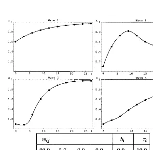
Thus, for our artificial networks, if the starting values were chosen such that wave 1 had the highest expression level at the first point in time, the dynamics of the network, as shown in Fig. 1, was such that wave 1 reached high expression levels first, followed by wave 2 etc.
4.1. Single time series
The method of reverse engineering described in the previous section was applied to artificial expres-sion data obtained from the curves in the four upper panels of Fig. 1. Many runs were carried out for each of the two termination criteria defined in Section 3. There was no systematic difference in the
results obtained from the two criteria, and we chose to use the first criterion.
The results of the computer runs are shown in Table 1. Individual runs were stopped at f=0.9, corresponding to an average error ofs/3.swas set
to 0.1. As can be seen from the table, the results were of mixed quality: All of the weights that were supposed to be zero were correctly determined in the sense that the interval spanned by the corre-sponding standard deviation contained the value zero. Furthermore, all of the time constants were close to their correct values. On the other hand, of the ten weights that were supposed to be non-zero, only five were significantly non-zero, whereas the other five were not, and the standard deviation was rather large for most weights.
Table 1
Network obtained from a single time series of artificial expression data generated using the network in Fig. 1a
wij bi ti
1.8916 12915
16911 7.5917 2.095.6 9.591.1
−1395.8
aThe results shown are the average of 50 runs.
Table 2
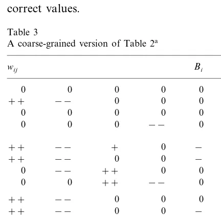
Results from runs with 30 data points per wave, distributed among one time series (upper table), three time series (second table), and five time series (third table)a
ti
wij bi
7.5912 0.80913 3.794.8
11911 7.8912 1191.2
0.45913 −2.4914
−1697.3 1.894.6
1497.7 7.591.8
6.1913 3.2914 1.995.8
5.9914 11911 9.190.73
5.3911 −1697.0 1.695.7
1.5913 1695.3
3.0911
9.996.6 −2.9912
1993.5 −1796.8 3.593.4 1190.28
−0.10912 0.08915
2292.2 −2194.3 1.291.8 1190.47
−1.398.1 3.2910
−1594.7 −5.992.0
1994.2 6.390.82
−1496.5
−2.393.0 1396.5 9.898.7 1.992.7 6.390.69
1693.9 −2293.9 −0.3592.7
aThe correct network, from which the artificial data was generated, is shown in the lowermost table.
4.2. Multiple time series
In the previous subsection, the data consisted of only one time series for each wave. In such a case, the data points follow a given trajectory in state space, and are not independent of each other. Thus, even if the curves in Fig. 1 had been sampled at twice as many points, the additional information obtained would not have been very large. Therefore, in order to add new information to the data set, it appears better to take a few measurements along different state space trajecto-ries rather than taking many measurements along one trajectory.
In order to test the effect of adding more time series to the data set, three sets of runs were carried out. In all three sets, 30 data points per wave were used. In the first set, the data points for every wave were all obtained from one single trajectory (time series). In the second set, ten points per wave were measured from each of three different trajectories, and in the third set, six points per wave were measured from each of five different trajectories.
table, the expression level curves were monotonous, containing only very little informa-tion to constrain the parameters. Adding two or four time series significantly improved the results (second and third tables), despite the fact that the total number of data points was unchanged.
Thus, for the first set of runs, only three of the weights were significantly non-zero, compared with eight in the correct network, and the stan-dard deviation was very large for most weights. None of the bias terms obtained significant non-zero values.
For the second set of runs, based on three time series of data (second table), all the weights that were supposed to be non-zero were indeed signifi-cantly different from zero, which also was the case for the set of runs based on five time series (third table). For the second set of runs, two bias terms were significantly non-zero, whereas all the bias terms were close to their correct values for the third set of runs, with only the second bias term being significantly different from zero. In both cases, the time constants were very close to their correct values.
When presented in the form used in Table 2, the results are far from transparent and also difficult to compare. In order to facilitate the comparison, the results are presented again, in a different form, in Table 3. Here, weights and biases are given as 0, positive (+), strong positive (+ +), negative (−), or strong negative (− −), with the boundary between positive (negative) and strong positive (negative) set, somewhat arbi-trarily, at 10 (−10). A weight is set to 0 if the interval formed by the standard deviation con-tains zero. Apart from making the comparison between different networks simpler, this form of presentation will also be more realistic when the results obtained from real data are displayed: with the measurement accuracy presently available, one does not expect (or need) to find exact weights and therefore a coarse representation, as used in Table 3, should be sufficiently accurate.
5. Application to rat spinal cord and hippocampal data
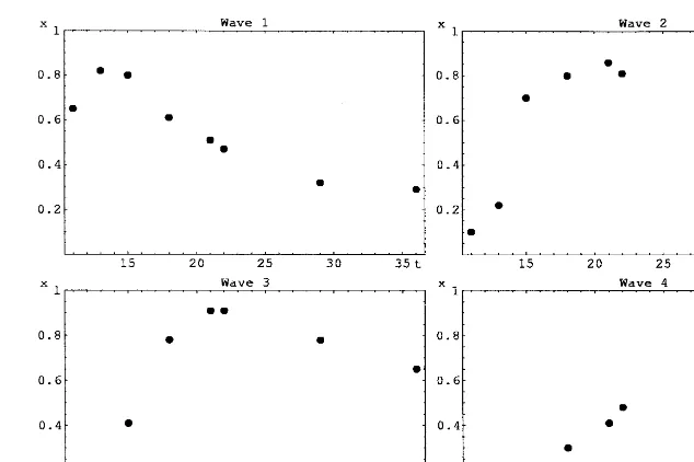
We have used the data obtained by Wen et al. (1998) for the development of rat spinal cord and hippocampus. The data consists of measurements for of order 100 genes for each tissue, with a total of 65 genes in common for the two tissues. Wen carried out a cluster analysis through which four distinct waves of expression and a constant wave were identified. With the constant wave included in the bias term, we were left with four dynamic variables. Wave 1 contains genes active during initial proliferation, wave 2 is associated with neurogenesis, wave 3 contains mostly genes for neurotransmitter signaling, and wave 4 is made up of genes active during the final maturation of the tissue.
The four waves of expression for the spinal cord data are shown in Fig. 2. Similar curves (not shown) were also obtained for the hippocampal data. We made three sets of runs, fitting network parameters to spinal cord data (set 1), hippocam-pal data (set 2), and both data sets together (set 3). For data obtained in different tissues, one must also include the possibility of a systematic difference between the networks describing the Table 3
A coarse-grained version of Table 2a
ti
aThe panels show the data from the runs with one time
Fig. 2. Expression levels for the four waves identified by Wen et al. (1998). For each panel, the horizontal axis shows time (in days), and the vertical axis the expression level, computed as an average of the expression levels of the genes in the corresponding cluster. different tissues. Thus, in set 3 we included, for
each wave, a tissue dependent parameter ti, and used the network equations
tix;i+xi=g
ati+bi+%j
wijxj
, i=1,…, 4 (5)where a is equal to −1 for the spinal cord data
and +1 for the hippocampal data.
The runs in set 1 and 2 were terminated when the average error was 0.7s, and the runs in set 3
were terminated at an average error of 0.9s, with
s=0.1. The results of the three runs are shown in
Table 4. Set 1 and set 2 gave almost identical results for the first two waves, i.e. fori=1 and 2, but conflicting results for the last two waves. It is reassuring to note that the results of set 3 agreed quite well with those of sets 1 and 2 in the case of the first two waves. As was the case for the artificial data, the standard deviation of the parameters decreased when additional time series were used, and so, for set 3, several of the biases obtained significant non-zero values. Note, how-ever, that the biases obtained from set 3 cannot be compared directly with those obtained from sets 1 and 2, due to the inclusion of the ti parameters, whose coarse-grained values are also given in the
table corresponding to set 3. We note also that the time constants agree rather well for all three runs. Thus, from Table 4 we can say with some confidence that wave 4 has an inhibitory effect on wave 1, and that wave 1 has an excitatory effect on wave 2. With slightly less confidence, we con-clude that wave 1 has an excitatory effect on wave 3, and that both waves 3 and 4 have an inhibitory
Table 4
Results from the three sets of runs carried out with real dataa
ti
ti
bi wij
0 0 0 −− 0 14
0 0
++ 0 0 5.1
−− 0 5.2
0 ++ 0
17
++ 0
−− 0 0
0 0 0 −− 0 19
++ −− 0 0 0 9.4 7.0 0 0
−−
0
++
0 0 −− 0 16
++
0 0
0 −− ++ 18 +
−− −
++ 0 0 + 6.2
0 7.1
++
0
++ 0 −−
0 ++
0 −− 0 18 0
effect on themselves. Finally, we also note that a number of the interactions are rather weak.
6. Conclusion and further work
We have introduced and evaluated the perfor-mance of a method for reverse engineering of genetic regulatory networks, and applied it to artificial data sets as well as to a coarse-grained representation of a data set consisting of mea-surements from rat central nervous system.
The evaluation shows that, for N4, the method is able to obtain an accurate representa-tion of the parameters of a network, provided that there are measurements from several time series available. With only one time series of data, some features of the network can still be determined, albeit less accurately.
The next step in our analysis will be to apply the procedure described in this paper to systems with different N and larger data sets, and to improve the speed and accuracy of the method by, for example, allowing the GA to vary dy-namically the connectivity of the network.
References
D’Haeseleer, P., Wen, X., Fuhrman, S., Somogyi, R., 1999. Linear modeling of mRNA expression levels during CNS development and injury. In: Altman, R.B., Dunker, A.K., Hunter, L., Klein, T.E., Lauderdale, K. (Eds.), Pacific Symposium on Biocomputing ’99. World Scientific, Singa-pore, pp. 41 – 52.
Davis, L. (Ed.), 1991. Handbook of Genetic Algorithms. Van Nostrand Reinhold, New York.
Holland, J.H., 1992. Adaptation in Natural and Artificial Systems (1st edn.: University of Michigan Press, Ann Arbor, 1975), 2nd edn. MIT Press, Cambridge.
Kauffman, S.A., 1993. The Origins of Order: Self-Organiza-tion and SelecSelf-Organiza-tion in EvoluSelf-Organiza-tion. Oxford University Press, Oxford.
Mitchell, M., 1996. An Introduction to Genetic Algorithms. MIT Press, Cambridge.
Reinitz, J., Sharp, D.H., 1995. Mechanism of eve strip forma-tion. Mech. Dev. 49, 133 – 158.
Somogyi, R., Sniegoski, C.A., 1996. Modeling the complexity of genetic networks: understanding multigenic and pleiotropic regulation. Complexity 1, 45 – 63.
Wen, X., et al., 1998. Large-scale temporal gene expression mapping of CNS development. Proc. Natl. Acad. Sci. 95, 334 – 339.
Yuh, C.-H., Bolouri, H., Davidson, E.H., 1998. Genomic cis-regulatory logic: experimental and computational anal-ysis of a sea urchin gene, Science 279, 1896 – 1902.