International Review of Economics and Finance 8 (1999) 131–146
Contagious bank runs
Spiros Bougheas*
Division of Economics, Staffordshire University, Leek Road, Stoke-on-Trent ST4 2DF, UK
Received 4 August 1997; accepted 11 June 1998
Abstract
We present a model of the propagation process of bank runs. A bank failure alone is not sufficient to trigger a panic. In accord with the empirical evidence, runs become contagious only during periods of macroeconomic instability. In addition, we make a clear distinction between illiquidity and insolvency as possible causes of bank failures. We also show that, despite the possibility of runs, the deposit contract is superior to autarky. 1999 Elsevier Science Inc. All rights reserved.
Keywords:Bank runs; Illiquidity; Insolvency
1. Introduction
Since the early 1980s we have witnessed a growing research interest in issues related to the stability of the banking system. One of the reasons the subject has attracted so much attention is because a bank failure, unlike the failure of another firm, is regarded as a possible threat to its competitors; it is believed to be contagious. However, as Kaufman (1988) and Park (1991) have recognized, despite the large volume of work on bank runs, the process by which these develop into runs on the whole banking system has not received a rigorous treatment. Existing models, which are essentially models of the banking system, treat all banks symmetrically.1 Understanding the
propagation process, however, requires that we distinguish between the banks respon-sible for causing the panic and those afflicted by the ensuing run.
The empirical evidence provides some useful suggestions concerning the causes of bank runs.2Rolnick and Weber (1984) find, contrary to common belief, that, during
the Free Banking Era in the United States (1837–1863) the banking system was not more unstable than later periods. Hasan and Dwyer (1994) provide evidence indicating the existence of contagious bank runs during the Free Banking Era that were caused
* Corresponding author. Tel.:144-1782-294-140; fax:144-1782-747-006.
E-mail address: [email protected] (S. Bougheas)
by events exogenous to the banking system. Furthermore, evidence from the National Banking System (1863–1913) indicates that periods of bank failures were associated with macroeconomic instability (e.g., Bernanke, 1983; Friedman & Schwartz, 1963; Gorton, 1988; and Kaufman, 1994). During this period, banks established a network of clearinghouses which was responsible for the supervision of the banking industry.3
One of the services offered by the clearinghouses was the provision of emergency assistance to banks facing liquidity problems. This system came to an end in 1913 with the establishment of the Federal Reserve System.
The majority of the empirical evidence on bank runs is concentrated on the early Great Depression. While the study by Saunders and Wilson (1996) covers the whole pe-riod from 1929 to 1933, the study by Calomiris and Mason (1997) concentrates on the June 1932 Chicago banking panic. Both studies find strong contagion effects; they also stress, however, the significant role of economic shocks. In addition, both studies support the information hypothesis of bank runs (Chari & Jagannathan, 1988; Jacklin & Bhatta-charya, 1988). According to this hypothesis, uninformed depositors run against solvent banks upon receiving a noisy indicator. After examining the evidence from the 1932 Chicago panic, Calomiris and Mason (1997) argue that, “the panic was caused by fears of bank insolvency, rather than by exogenous liquidity demand by depositors” (p. 868). In contrast, the model of Diamond and Dybvig (1983) presents bank runs as “sunspot” equilibria; in other words, they are the “bad” outcome of a coordination game.
In this article, we present an infinite horizon, overlapping generations version of Jacklin and Bhattacharya’s (1988) model of information-based runs.4Members of each
generation live three periods, but enjoy consumption only in the last two periods. Agents can either store their endowment or invest it in a risky, irreversible, two-period technology. When they are born, agents are uncertain about their future preferences for their life-time consumption patterns. Therefore, the generation-specific role of banks in this environment is to offer agents insurance against this idiosyncratic preference risk by pooling their resources together. Contagion is introduced through serial correlation across bank returns over time. Each bank’s return depends on both the state of the economy and the return of the bank established one period earlier. The possibility of a bank run arises because we assume that the terms of the banking contract are not contingent on the solvency status of other banks.
The above framework captures the flow of information across the banking system and thus allows us to examine the repercussions of a bank failure on the financial status of other banks. The process begins when the market value of a bank’s assets (loans) falls below that of its liabilities (deposits) (i.e., when it becomes insolvent). At this point, the reaction of depositors is crucial. If they fear that all banks are subject to the same shock, then they will attempt to withdraw their funds, thereby creating liquidity problems for other banks. If this possibility of contagion exists, we need to examine carefully what leads depositors to believe that other banks are also in danger of becoming insolvent.
corre-lated. Depositors using this information update their beliefs about the financial status of other banks. When their new assessment assigns a high probability of bank insol-vency, they rationally decide to withdraw the funds from their accounts. In this case, all banks face a liquidity problem.
Of course, the depositors’ assessment can be wrong. It is possible that the banks experiencing the run are solvent. In imperfect capital markets the distinction between insolvency and illiquidity is crucial. Solvent banks facing liquidity problems are forced, in the absence of any intervention, either to sell their illiquid assets or to borrow. Premature liquidation of assets could force their market value below their book value, leading the bank to insolvency. These are the considerations which prompted Bagehot5
(1873) to suggest that central banks should extend emergency assistance to illiquid, but not insolvent banks.6In our model, it is shown that, during periods of economic
instability, solvent banks can indeed face liquidity problems caused by the reaction of depositors to news about the financial insolvency of other banks.
Despite the possibility of a panic we also show that bank deposits can offer a higher expected return than autarky.7Under autarky each agent makes investment decisions
separately (no pooling of funds). In other words, the runs in our model are equilibrium phenomena (Postlewaite & Vives, 1987).
In the following section, we present a slightly altered version of the Jacklin and Bhattacharya (1988) model (hereafter JB). In section 3, we develop the overlapping generations framework, and in section 4, we present an example using specific func-tional forms. In section 5, we calibrate the model to demonstrate the superiority of the banking contract to autarky.
2. The JB model
What follows is a slightly altered version of JB. There is a continuum of agents born att50 who live for three periods, t50, 1, 2. Each agent is endowed with one unit of the single divisible homogeneous good and two investment technologies. Let
xdenote the amount invested in these technologies. The first technology, which can be represented by the triplet (2x,gx, (12 g)x), where 0< g <1 denotes the amount withdrawn in the first period, is a simple storage technology.8The second technology,
which can be represented by the triplet, (2x, 0, R˜ x), is an irreversible (illiquid) technology that in the third period offers a random rate of return, R˜ . The realized value, R, which becomes publicly known at t 5 2, takes the value L with prior (at
t50) probabilityp and the valueHwith probability 12p, where 0,L ,H.
All agents are identical att50 and derive utility from consumption att51 and
t52. Att51 they learn their type, which remains private information. The preferences of typej(j51, 2) are described by [Eq. (1)]:
Vj(c1, c2)5 U(c1) 1 bjU(c2), (1)
where bj denotes the discount factor for type j. It is assumed that 0 , b1 , b2 5
1.9 There is no aggregate uncertainty about liquidity demand in this economy and
2.1. The deposit contract
The role of banks is to provide insurance to agents against their idiosyncratic liquidity risk and allow them to take advantage of the higher expected return of the illiquid technology whose risk is systematic. LetctjRdenote consumption by typejat
t, conditional on R for t5 2, and let D denote the amount invested in the storage technology. Then, as JB shows, the optimal contract can be found as a solution to the following social optimization problem [Eq. (2)]:
max
tjR pV1(c11, c21H,c21L) 1 (12 p)V2(c12, c22H, c22L) (2)
subject to:
D> pc11 1(12 p)c12 (3a)
R(12 D) > pc21R1(12 p)c22R∀R (3b)
V1(c11,c21H, c21L) >V1(c12, c22H,c22L) (4a)
and
V2(c12,c22H, c22L) >V2(c11, c21H,c21L) (4b)
Eqs. (3a) and (3b) represent the second and third period resource constraints. Eqs. (4a) and (4b) are the self-selection constraints, whereV1(c12,c22H,c22L) and V2(c11,c21H, c21L) represent the utility from which types 1 and 2, correspondingly, will derive if
they misrepresent their true types. Notice that the value of g has been set equal to one in the resource constraints. As we show in Appendix 1, under autarky no type will choose to use the storage technology in the third period. As a consequence, the optimal value ofgfor the above problem is also equal to one. The reason for making the storage technology available in the third period is to allow banks to hold excess reserves. Finally, letc*jtRdenote the optimal allocation.
3. The Overlapping Generations model
Because our objective is to show how a single bank failure can trigger runs on other banks, our model needs to capture the transmission of information across the banking system. With this goal in mind, we choose the overlapping generations (OLG) framework, which allows us to model explicitly the flow of information from one bank to another.10We consider an infinite horizon, overlapping generations version of the
JB model,t51, 2, . . . . At the beginning of each period a new bank is created, each being essentially identical to the one examined in JB. Let b(t) denote the bank established by members of the generation born at t and R˜t the gross return on its
illiquid investment.11We do not allow any intergenerational (interbank) lending. To
3.1. Information structure
According to Gorton’s (1988) empirical study, bank panics are events linked to the business cycle: “The recession hypothesis best explains what prior information is used by agents in forming conditional expectations. Banks hold claims on firms and when firms begin to fail, a leading indicator of recession (when banks will fail), depositors reassess the riskiness of deposits” (p. 778). In our model, during periods of recession, when the firm failure rate is high, the asset returns across the banking system are highly correlated. This assumption is consistent with the evidence provided in Calomiris and Mason (1997) on the June 1932 Chicago panic, “failures during the panic reflected the relative weakness of failing banks in the face of a common asset value shock . . .” (p. 881). During each period the state of the economy is represented by a first-order Markov process that specifies next period’s return distribution of banking assets conditional on this period’s realized return. From an empirical perspective the “state of the economy” might represent a variety of economic variables. For example, Calom-iris and Mason (1997) argue that the June 1932 Chicago panic was triggered by several factors, such as the falling prices of corporate assets, a municipal revenue crisis, and a case of bank fraud.
We assume that all members of each generation receive the same information and update their expectations in the same way.12During each period, depositors receive
the following two information signals: a) the realized return of the bank established two periods earlier; and b) the state of the economy. For periodt, the two signals are described by the pair (st, St). st P {L, H} indicates the realization of R˜t22 (i.e., the
investment return of the bank established two periods earlier). St P {S1, . . . , Sn}
describes the state of the economy. Let
Pi;prob(St5Si),
o
ni51Pi5 1.
Notice that both the set of states of the economy and their corresponding probabilities are time-independent. Each Si, (i5 1, . . . , n), is a first-order Markov process, that specifies the probability distribution of R˜t21 conditional on st(i.e., the realization of R˜t22). Let
prob(R˜t215 k|st5m and St5Si) (5)
wherek5L,Handm5L,Hdescribe the probability distribution of the asset return of the bank established one period earlier,b(t21), conditional on both the realized return of the bank established two periods earlier, b(t 2 2), and the state of the economy att.The probabilities in Eq. (5) must satisfy the following condition:
prob(R˜t215 L|st5m and St5Si) 1prob(R˜t215H|st5m
and St5 Si) 51, ∀mand ∀i.
It is also assumed that the two signals are independently distributed.13
At each t, before members of each generation make any decisions, they observe the two signals, (st, St).14 Given this information, members of b(t2 1) update their
ofb(t), the new bank, use this information to calculate their prior probability distribu-tion of R˜t by using the following rule [Eq. (6)]:
pt;prob(R˜t5L) 5{
o
ni51Piprob[R˜t5L|R˜t215H, St115Si]}
3prob(R˜t215H|st,St) 1{
o
ni51Piprob[R˜t5L| R˜t21 5L,St115Si]}
3prob(R˜t215L|st,St) and 12pt;prob(R˜t5H) (6)
At periodt, members ofb(t) know that att11 they will learn the two signals (st11, St11) and update their prior beliefs about the asset return distribution of their bank
using Eq. (5) (carried one period forward). Therefore, at timet, they form their prior beliefs by calculating the expected value of Eq. (5) by taking into account that there aren32 possible pairs of signals. They also use their knowledge of the current state of the world to calculate the probability distribution of the asset returns ofb(t21). Because banks and depositors form expectations in the same way, these are also the probabilities that banks use when they design the deposit contracts.
We impose the following restriction:
o
ni51Piprob[R˜t5L |R˜t215H, St115Si] 5
o
ni51Piprob[R˜t
5L |R˜t215L,St115 Si].
The economic interpretation is that the signal st11(the observation of Rt21) alone is
uninformative. In other words, the state of solvency of a particular bank is not sufficient to cause depositors at other banks to update their beliefs about the financial status of their own bank. What is required is the dual observation of that signal and the state of the economy. We are going to show that even if the above restriction holds, bank runs can still be contagious when the economy is in a recession.
3.2. The contract
Given the informational structure of the model an ex ante optimal contract forb(t) at time t would require the bank to offer payments which are contingent on (st11, St11) (i.e., the following period’s realizations of the two signals). If it was indeed
possible for the banks to offer such contracts then these contracts would never cease to be incentive compatible and thus information-based runs would never take place. However, this type of contract would involve enormous computational difficulties.15
Furthermore, their design would presume that courts would not have any problems enforcing contracts with terms contingent on the performance of other banks.16
With the above in mind, we find the solution for the deposit contract by maximizing Eq. (2) subject to Eqs. (3) and (4), where here Eq. (6) is used for the calculation of
pt. If at t11
prob(R˜t5L|st11, St11) ?pt
deposit contract they realize that for some future states the bank will not be able to meet its obligations.
It is crucial at this point to make clear that we do not assume that depositors are able to use information better than the banks. Both sides know that, given the contract offered, there is always a possibility of a bank run and both parties can calculate the allocations which the contract offers at each state. What we argue is that when depositors decide whether or not to deposit their funds at the bank they take into account that there is a possibility that they will not receive the allocation specified by the contract. A bank run is always a possibility. Therefore, their expected utility from the deposit contract att, is given by Eq. (7):
V* 5
o
(n32)
prob(st115m and St115Si) [pV1(c11,c21H, c21L| (m,Si)
1(1 2 p)V2(c12, c22H,c22L|(m, Si)], (7)
wherem5 L,H, and prob(st11 5mand St115 Si) 5prob(st115 m) 3 Pibecause
the two signals are independently distributed. The expression in the brackets describes their expected utility from the same contract one period later,t11, given that they will receive the signal (st11,St)5(m,Si). If the signal means that their ex post beliefs
differ from their prior beliefs then the allocation which they will receive might differ from the one specified by the contract (i.e.,c*tjR). For those signals where their ex post
beliefs equal their prior beliefs, i.e., prob(R˜t 5L|st11, St11) 5pt
their expected utility is given by:
pV1(c11,c21H, c21L| (m,Si) 1(12 p)V2(c12,c22H, c22L |(m,Si))
5 pV1(c*11, c*21H,c*21L) 1(1 2 p)V2(c*12, c*22H, c*22L).
If the expression in Eq. (7) is greater than the expected utility derived from autarky, then the depositors will accept the deposit contract even if there is a possibility of a bank run.
4. An example
Following JB, letU(c)5
√
c, 0, b1, b251. After substituting the above expressionsin Eq. (2) and Eq. (4), and noticing that only Eq. (4a) is binding, we obtain the following solution for the bank’s problem:17, 18
c*11 5
1
p(11 b2A2H) 1(12 p)(K2
11A2K22H)
,
c*12 5K21c*11,
c*21H5(AbH)2c*11,
c*21L5c*21H(L/H),
c*22H5(AK2H)2c*11,
where
A5(1 2p) 1p(L/H)1/2,
K15
11 bA2H[b 2 p(12 b)]
11 bA2H[12 p(12 b)]
K25
11 b2A2H[12 p(12 b)]
1 1 bA2H[12 p(12 b)].
As JB suggest, we can interpret the above allocations as follows: ifR 5Hthen the bank is considered solvent and pays at the end of the second period its promised payments,c*21Hand c*22H; if R 5 L then the bank is considered insolvent and it pays L/Hof its promised payments. The above allocation satisfies the following conditions:
c*11. c*12, c*21R, c*22R, R5L, H.
4.1. Bank Runs
With their updated priors in the second period, depositors might be able to improve their individual well-being by misrepresenting their types. The next step is to find under what conditions the above allocation ceases to be incentive compatible.
Define prob(R˜ 5L|s,S);p9. Suppose the posterior beliefsp9 given the realized state (s,S), are not equal top.Then the following expressions describe the conditional expected utility for the two types given that they reveal their true preferences:
EU(type 1)5{1 1 b2(12 p9)AH 1 b2p9AH(L/H)1/2} (c*
11)1/2, (8)
EU(type 2)5{K11(12p9)AHK21 p9AKH2(L/H)1/2} (c*11)1/21. (9)
LetA9 ; (1 2 p)9 1 p9(L/H)1/2. Then Eqs. (8) and (9) can be rewritten as Eqs.
(89) and (99):
h
1 1Ab2A9Hj
(c*11)1/2 (89)
h
K11AK2A9Hj
(c*11)1/2 (99)Eq. (4a) which is the binding self-selection constraint can be written as Eq. (10):
11 b(1 2p)AbH1 bpAbH(L/H)1/2
5K11 b(12p)AHK21 bpAHK2(L/H)1/2,
or
(12K1) 5 bA2H(K22 b). (10)
Proof: From Eqs. (8) and (9), type 2 depositors will pretend to be type 1, if
K11 AHK2A9 ,1 1AbHA9
or
1 2K1.AHA9(K22 b).
Substituting Eq. (10) for the left-hand side of the above expression we get the desired result.
The above condition is satisfied for relatively high values ofp9. Because the posterior probability of bank insolvency is high, type 2 depositors prefer allocations which allow them higher early withdrawals. Given thatc*11. c*21, the bank will be unable to meet
all withdrawal demands. Therefore, it is assumed that the bank, which cannot distin-guish among types, will serve depositors on a first-in, first-served basis. That means that each depositor gets the type 1 allocation with probability p. Therefore, the expected utility of each type under this arrangement is given by:
EU(type 1)5
5
p3
1 1 b2A9AH4
1 (12 p)3
K11 bK2A9AH
46
(c*11)1/2,and
EU(type 2)5
5
p3
1 1 bA9AH 1 (12 p)3
K11K2A9AH46
(c*11)1/2.The next result shows what happens when the posterior probability of bank insol-vency is low. In this case, type 1 depositors pretend to be type 2, since the higher expected return compensates them for their impatience.
RESULT 2: IfA,A9, then the type 1 allocation will not be incentive compatible. Proof: From Eqs. (8) and (9), type 1 depositors will pretend to be type 2, if
1 1Ab2HA9 ,K
11AHK2bA9
or
1 2K1,AA9bH(K22 b).
Substituting Eq. (10) for the left-hand side of the above expression we get the desired result.
The above condition is satisfied for everyp9 , p.Since type 1 depositors believe that the probability of bank insolvency is low, they prefer to leave their funds at the bank for one more period and take advantage of the higher expected return on the bank’s assets. In this case the excess reserves,p(c*11 2c*12,), will stay at the bank
until the end of the second period, when the bank is liquidated and all remaining funds are divided equally among the depositors, each one receiving p(c*112 c*12) 1
f
pc*21R1(12 p)c*22Rg
, where the second term denotes the total return from the illiquidtechnology.19 Then the expected utility of typejdepositor given this arrangement is
(c*12)1/21 bj
5
(12p9)3
p(c*11 2c*121c*21) 1(12 p)c*224
1/21
p9
3
p(c*112 c*12 1c*21(L/H))1(12 p)c*22(L/H)4
1/26
.Let us take a closer look at the two results. Because the prior beliefpis a weighted average of all possible posterior beliefsp9, [see Eq. (6)], there will be at least one p9
such that type 1 depositors will pretend to be type 2. However, this does not cause any problems for the bank. On the other hand it is possible that for some states, type 2 depositors will prefer the type 1 allocation. In these states the bank will be unable to meet the demand for liquidity. These are the important states for our study. As depositors learn the state of the economy and observe the solvency status of those banks established one period earlier, they update their beliefs about the distribution of returns of their own bank. After observing that banks established one period earlier become insolvent and that the state of the economy indicates a positive correlation among the returns in the banking system, depositors conclude that the probability that their own bank will become insolvent has increased. As both types attempt to make high withdrawals the banks reserves are depleted. The run is caused by factors not directly related to the bank’s financial performance and the bank is facing liquidity problems without being necessarily insolvent.
4.2. Autarky
The following program gives the solution for the autarkic equilibrium:
V*a 5max
1, 2
p
5
(c1)1/2 1 b(c2)1/2A6
1(12 p)5
(c1)1/21(c2)1/2A6
subject to:
c11c2/H 51,
where we defined, c2H; c2and c2L ;c2 (L/H). The above formulation is consistent
with the available technologies, because, as we show in Appendix 1, agents never choose to invest in the storage technology in the third period. LetB;pb 1 (12 p). Then we obtain the following solutions:
c*1 5
1
1 1HA2B2, c*2 5
H2A2B2
1 1HA2B2.
5. Numerical examples
In this section we present numerical examples which compare the performance of the deposit contract as given by Eq. (7) to that of autarky. In all examples the following parameters remain constant: p 5 0.5,b 5 0.8, p 5 0.4, pL 1 (1 2p)H 51.4 and
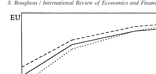
Fig. 1. Expected utility derived from the deposit contract and autarky as a function of asset return variability. A, solid line; C1, dotted line; C2, dashed line.
We are interested in three types of experiments. The first concerns the responses of the deposit contract and autarky to changes in the variability of the risky asset return. Keeping the mean constant, we have considered the following values forL: 0.5, 0.8, 1.1, 1.4. The second experiment involves a variation in the probability distribu-tion of the three states of the economy keeping the transidistribu-tional probability matrices (i.e., the correlation in asset returns across banks) constant. More specifically define
Si;ppi(L|L) pi(L|H) i(H|L) pi(H|H).
Siis the transitional probability matrix for statei, (i51, . . . ,n). Then let
S15
0.8 0.6
0.2 0.4, S25
0.4 0.4
0.6 0.6, S3 5
0.0 0.2 1.0 0.8.
S1signals “bad” news—not only that the posterior probability of insolvency is high,
but that probability is even higher when other banks are insolvent. At the other extreme,S3signals “good” news about the economy in general and banking in
particu-lar.20 Notice that at S
2the posterior probability distribution is the same as the prior
one.
Fig. 1 shows the results of these two experiments. The C1 line (dotted line) shows the variation in the expected utility derived from the deposit contract as L takes different values andP150.2,P250.6, andP350.2. The C2 line (dashed line) shows
the same relationship for P15 0.1, P25 0.8, and P35 0.1. The A line (solid line)
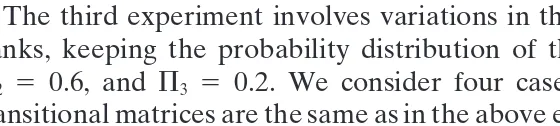
Fig. 2. Expected utility derived from the deposit contract and autarky as a function of the correlation in asset returns across the banking system. A, solid line; C, dashed line.
The third experiment involves variations in the correlation in asset returns across banks, keeping the probability distribution of the three states the same, P1 5 0.2,
P2 5 0.6, and P3 5 0.2. We consider four cases. For case a the three probability
transitional matrices are the same as in the above example. The corresponding matrices for casesb and c are shown below:
b: S15
0.8 0.4
0.2 0.6, S25
0.4 0.4
0.6 0.6, S35
0.0 0.4 1.0 0.6,
c: S1 5
0.6 0.4
0.4 0.6, S25
0.4 0.4
0.6 0.6, S35
0.2 0.4 0.8 0.6.
For casedthe returns are not correlated. Notice that as we move from caseato case dthe degree of correlation decreases.
Fig. 2 shows the results. Notice that because the above changes do not affect the autarkic equilibrium theAline (solid) is horizontal. However, as we move fromato dthe deposit contract [Cline (dashed)] performs better since the correlation of bank returns in the “bad” state gets weaker.
6. Concluding comments
In this paper, we have presented an OLG model of the propagation process of bank runs. Instead of using the OLG framework we could have developed a simple three-period multi-bank model. The benefit of the additional complexity, however, is that the OLG framework treats all banks symmetrically. In a three-period model all banks would be subject to an aggregate shock, but only one bank’s depositors would receive interim information about the shock. As other depositors observe a run at the bank with the informed depositors, they might attempt to close their own accounts, depending on their beliefs about the correlation between bank returns. The overlapping generations framework avoids this asymmetry. There is noa priori
in the state of the economy can lead to a bank panic. We have shown that under certain conditions—in an unregulated environment—bank runs can be contagious. Before we reach any policy conclusions we need to examine carefully the following two issues.
The first issue is related to the causes of bank panics. Does the possibility of a run on one bank causing a run on other solvent banks necessarily mean that the banking system is inherently unstable? The answer is negative. In our model, bank runs become contagious only during periods of economic downturns. The shape of the economy determines whether bank runs will spread throughout the system.
The second issue addresses directly the external effects of a bank failure. Even if an insolvent bank alone cannot trigger a widespread panic, it still sends a signal that, during a period of macroeconomic instability, can have adverse effects on other banks. These banks will face a liquidity shortage and, unless they manage to overcome it, they can become insolvent. In our model, to keep the analysis simple we have assumed that the long-term technology is irreversible. Following Diamond and Dybvig (1983), we can let this technology be only partially irreversible, thus capturing the effects of imperfect capital markets on the value of banking assets. In this situation, suspension of convertibility of deposits into currency can provide time to solvent banks to work out their liquidity problems. After all, this is exactly the policy that banks have followed during the National Banking System with the help of privately established clearinghouses.
Appendix 1
We show that under autarky depositors will not invest in the storage technology at the end of the first period. Let (12p)H21/21pL21/2,1 andB2A2H>1, conditions
satisfied by the numerical example.
If we solve the optimization problem for type 1 depositors, we can establish an upper bound for the investment in the storage technology, since these depositors have the higher discount factor (lowerb). The optimal solution of this problem requires:
(1 2c*1)/c15B2A2H>1,
where (12c1)His substituted forc2. Thenc*1,0.5, is the desired upper bound. Notice
thatc1denotes the amount invested in the storage technology at the beginning of the
first period which is not necessarily equal to first period consumption.
Next consider the expected utility of type 2 depositors at the end of the second period. Let 0< d <c*1, denote the amount they will invest in the storage technology
at the end of the first period. If we can show thatd 50 when c150.5 then d must
be equal to 0 for anyc*1 , 0.5. The expected utility of type 2 depositors whenc1 5
0.5, is given by:
(0.5 2 d)1/21(12p)
3
0.5H 1 d4
1/2 1p3
0.5L1 d4
1/2;W(d).Given that (12p)H21/21pL21/2,1, it is straightforward to show that W9(0),0.
Acknowledgments
Paper presented at the meetings of the Northern Universities Macro Research Group at Liverpool John Moores University, UK, February 1995. I would like to thank four referees, Nick Adnett, Eric Bond, Kevin Dowd, Brian Hillier, Derek Laing, and John Whittaker for their helpful comments. All remaining errors are mine.
Notes
1. The literature took off after Diamond and Dybvig (1983) formalized the ideas in Bryant (1980). See also the work of Bhattacharya and Gale (1987), Chari and Jagannathan (1988), Drees (1992), Engineer (1989), Freeman (1988), Hau-brich and King (1990), Jacklin (1987), Jacklin and Bhattacharya (1988), Loewy (1991), Qi (1994), Smith (1984), and Williamson (1988).
2. For an historical perspective on bank runs, see Sprague (1910) and Smith (1991). Reviews of the empirical evidence are provided by Kaufman (1994) and Park (1991). Benston and Kaufman (1996) and Dowd (1996) discuss the stability of the banking system before the establishment of the Federal Reserve System. 3. Timberlake (1984) traces the development of clearinghouses and analyzes their
role in Central Banking.
4. See Temzelides (1997) for a multi-bank version of the Diamond and Dybvig (1983) model.
5. Cited in Schnadt and Whittaker (1992).
6. Preventing the insolvency of the banking system also led President Roosevelt in 1933 and, more recently, the governors of Ohio and Maryland in 1985 to declare bank holidays, thus postponing the convertibility of deposits into cur-rency. However, Wigmore (1987) argues that the objective of the bank holiday of 1933 was not to postpone the convertibility of deposits into currency but to protect the banking system from running out of gold.
7. For simplicity, we compare the performance of the deposit contract to autarky instead of to the market for equity shares considered by Jacklin and Bhatta-charya (1988).
8. In Jacklin and Bhattacharya (1988) the storage technology is not available in the third period.
9. Given this assumption, it is convenient to drop the subscripts and defineb1;b.
10. Freeman (1988), Loewy (1991), and Qi (1994) are other examples of banking models which use the overlapping generations framework.
11. Following Freeman (1988), we assume a sequence of finite-lived banks (i.e. a bank is generation specific).
12. Heterogeneity of agents with respect to the information structure is considered in Chari and Jagannathan (1988) and JB.
14. Notice thatb(t22) is liquidated att; therefore, this information is irrelevant for its depositors.
15. In our model the dimension of (st,St) is equal to 2 3n for everyt.
16. Our approach of assuming that variables are observable, but not contractible, follows the work on incomplete contracts; see Aghion and Bolton (1992). 17. To simplify notations, we drop the time subscripts.
18. Because of a typographical error in JB the expression forK2is slightly different.
19. This is possible because, contrary to JB, here it is assumed that the storage technology is available in the third period.
20. The slight negative correlation between the returns in S3offsets the positive
correlation in S1so that the signals remains uninformative.
References
Aghion, P., & Bolton, P. (1992). An incomplete contracts approach to financial contracting.Review of Economic Studies 59, 473–494.
Bagehot, W. (1873).Lombard Street.London: John Wiley & Sons.
Benston, G., & Kaufman, G. (1996). The appropriate role of bank regulation.Economic Journal 106, 688–697.
Bernanke, B. (1983). Nonmonetary effects of the financial crisis in the propagation of the Great Depres-sion.American Economic Review 73, 257–276.
Bhattacharya, S., & Gale, D. (1987). Preference shocks, liquidity, and central bank policy. In W. Barnett & K. Singleton (Eds.),New Approaches to Monetary Economics (pp. 69–88). New York: Cambridge University Press.
Bryant, J. (1980). A model of reserves, bank runs, and deposit insurance.Journal of Banking and Finance 4, 335–344.
Calomiris, C., & Mason, J. (1997). Contagion and bank failures during the Great Depression: the June 1932 Chicago banking panic.American Economic Review 87, 863–883.
Chari, V., & Jagannathan, R. (1988). Banking panics, information, and rational expectations equilibrium.
Journal of Finance 43, 749–763.
Diamond, D., & Dybvig, D. (1983). Bank runs, deposit insurance, and liquidity.Journal of Political Economy 91, 401–419.
Dowd, K. (1996). The case for financial laissez-faire.Economic Journal 106, 679–687.
Drees, B. (1992). Financial institutions or asset markets: alternative trading and banking arrangements as risk sharing mechanisms.European Journal of Political Economy 8, 175–200.
Engineer, M. (1989). Bank runs and the suspension of deposit convertibility. Journal of Monetary Economics 24, 443–454.
Freeman, S. (1988). Banking as the provision of liquidity.Journal of Business 61, 45–64.
Friedman, M., & Schwartz, A. (1963).A Monetary History of the United States 1867–1960.Princeton: Princeton University Press.
Gorton, G. (1988). Banking panics and business cycles.Oxford Economic Papers 40, 751–781.
Hasan, I., & Dwyer, G. (1994). Bank runs in the free banking period.Journal of Money, Credit, and Banking 26, 271–288.
Haubrick, J., & King, R. (1990). Banking and insurance.Journal of Monetary Economics 26, 361–386. Jacklin, C. (1987). Demand deposits, trading restrictions, and risk sharing. In E. Prescott & N. Wallace
(Eds.),Contractual Arrangements for Intertemporal Trade(pp. 27–47). Minneapolis: University of Minnesota Press.
Kaufman, G. (1994). Bank contagion: a review of the theory and evidence.Journal of Financial Services Research 8, 123–150.
Kaufman, G. (1988). Bank runs: causes, benefits, and costs.Cato Journal 7, 559–587.
Loewy, M. (1991). The macroeconomic effects of bank runs: an equilibrium analysis.Journal of Financial Intermediation 1, 242–256.
Park, S. (1991). Bank failure contagion in historical perspective. Journal of Monetary Economics 28, 271–286.
Postlewaite, A., & Vives, X. (1987). Bank runs as an equilibrium phenomenon. Journal of Political Economy 95, 485–491.
Qi, J. (1994). Bank liability and stability in an overlapping generations model.Review of Financial Studies 7, 389–417.
Rolnick, A., & Weber, W. (1984). The causes of free bank failures: a detailed examination.Journal of Monetary Economics 14, 267–292.
Saunders, A., & Wilson, B. (1996). Contagious bank runs: evidence from the 1929–33 period.Journal of Financial Intermediation 5, 409–423.
Schnadt, R., & Whittaker, J. (1992). A suggestion for the operating practices of the European Central Bank.Economies et Socie´te´s 9, 133–145.
Smith, B. (1984). Private information, deposit interest rates, and the ‘stability’ of the banking system.
Journal of Monetary Economics 14, 293–317.
Smith, B. (1991). Bank panics, suspensions, and geography: some notes on the ‘contagion of fear’ in banking.Economic Inquiry 29, 230–248.
Sprague, O. (1910).History of Crises under the National Banking System.Washington: U.S. Government Printing Office.
Temzelides, T. (1997). Evolution, coordination, and banking panics.Journal of Monetary Economics 40, 163–183.
Timberlake, R. (1984). The central banking role of clearinghouse associations.Journal of Money, Credit, and Banking 16, 1–15.
Wigmore, B. (1987). Was the bank holiday of 1933 caused by a run on the dollar?Journal of Economic History 47, 739–755.