monitoring forest degradation in tropical regions by

TROPICAL OPEN WOODLANDS SPECIAL ISSUE

Monitoring forest degradation in tropical regions by

remote sensing: some methodological issues

ERIC F. LAMBIN Department of Geography, University of Louvain, place Louis Pasteur, 3, B-1348 Louvain-la-Neuve, Belgium. Email: lambin@geog.ucl.ac.be

ABSTRACT comprehensive description of the surface processes.

The detection of inter-annual changes in landscape Key issues related to the monitoring by remote

spatial structure is more likely to reveal long term sensing of open forest degradation in a tropical

and long lasting land-cover changes, while spectral context are discussed. Degradation of forest-cover

indicators are more sensitive to fluctuations in is often a complex process, with some degree of

primary productivity associated with climatic ecological reversibility and a strong interaction with

fluctuations. Different monitoring systems may be climatic fluctuations. Only a representation of land

optimal for different ecosystems. A long time series cover as a continuous field of several biophysical

of observations is always required. The monitoring variables can lead to an accurate detection of forest

of the spatio-temporal distribution of biomass degradation. For this purpose, repetitive

burning may also give indications of open forest measurements of spectral, spatial and temporal

degradation. indicators of the land surface have to be performed.

Each set of indicators brings a specific type of Key words.Land-cover change, forest degradation, remote sensing, landscape, monitoring, tropical information on the land cover. These indicators

must therefore be combined to achieve a forest, deforestation, Africa.

observations on the vegetation cover at a regional scale.

INTRODUCTION

The lack of quantitative, spatially-explicit and statistically representative data on land-cover change Forest degradation is a process leading to a ‘temporary

or permanent deterioration in the density or structure of has left the door open to simplistic representations of forest-cover changes, for example, ‘marching deserts’ vegetation cover or its species composition’ (Grainger,

1993, p. 46). It is a change in forest attributes that or disappearing tropical forests. Whilst it is possible to find local examples of such extreme changes, empirical leads to a lower productive capacity. It is caused by

an increase in disturbances. The time-scale of processes studies in grassland, savannas or open forest ecosystems generally reveal the predominance of inter-annual of forest degradation is in the order of a few years to

a few decades. climatic variability, ecosystem resilience and complex land-cover change trajectories over secular land cover Any in-depth understanding of the processes of forest

degradation has to be based on an accurate monitoring conversions (Ringrose et al., 1990; Hellden, 1991; Tucker, Dregne & Newcomb, 1991; Prins & Kikula, of the degradation over large areas, for at least a few

decades. When it has to be performed at a regional 1996).

Previous studies generally distinguish between land-scale, this monitoring poses a number of

methodo-logical challenges. The objective of this paper is to coverconversion, i.e. the complete replacement of one cover type by another, and land-covermodification, i.e. discuss critical issues related to the monitoring of open

forest degradation in a tropical context through a more subtle changes that affect the character of the land cover without changing its overall classifica-review of recent studies on this topic. The emphasis

Eric F. Lambin

cover conversions. In principle, the monitoring of land- landscape heterogeneity. Variables such as vegetation community structure (e.g. tree:shrub:grass ratios), or cover conversions (e.g. agricultural expansion or

deforestation) can be performed by a simple species composition, cannot be observed reliably by remote sensing. In the following review, after a brief comparison of successive land cover maps, derived

either by classification of remote sensing data or by field discussion of different representations of land cover, the main options for the measurement by remote sensing of surveying. This change detection method is however

limited by the classification accuracy of the land cover indicators of the state of land-cover and its change are reviewed.

maps and, therefore, other change detection methods such as image differencing, change vector analysis, image regression or multi-temporal linear data

transformation are also applied (Coppin & Bauer,

DISCRETE VERSUS CONTINUOUS

REPRESENTATION OF LAND

1996).

In any case, the comparison of land-cover

COVER

classifications for different dates does not allow the

detection of subtle changes within land-cover classes. The land surface can be represented as a set of spatial units that are each associated with an attribute. These Even if some of the attributes of one class have changed,

the magnitude of these changes will not always be large attributes are either a single land cover category (i.e. leading to a discrete representation of land cover) or enough to justify a shift from one land cover category

to another, unless the vegetation classification identifies a set of values for continuous biophysical variables (i.e. leading to a continuous representation of land a very large number of narrowly defined categories.

Therefore, monitoring forest degradation can only cover) (DeFries et al., 1995). The correspondence between these two representations can be established be achieved through repetitive measurements of

bio-physical attributes that characterize the land cover. through a table which associates to each land cover category the average range of values for the biophysical These biophysical attributes must be surface

characteristics that are measurable from space, such variables. An example of such a table, which is based on the IGBP-DIS global land cover map at 1 km as vegetation cover, biomass, surface moisture or

Table 1. Table of correspondence between the IGBP-DIS land-cover classes for West Africa and key biophysical variables (see text for derivation).

Parameter Description BARR OPEN GRAS SAVA CROP WSAV EVG

z?? m(m) Roughness length for momentum 0.05 0.10 0.06 0.15 0.08 0.50 2.00

0.02–0.08 0.02–0.28 0.02–0.10 0.05–0.97 0.06–0.10 0.05–1.00 2.00–2.65

d(m) Displacement height / 0.70 0.70 0.35–7.00 0.70 0.35–7.00 14.00 LAI (−) Leaf Area Index 0.50 1.30 2.40 3.70 4.30 5.80 6.40

0.00–1.20 0.10–4.80 1.30–4.30 1.60–5.50 0.50–6.00 3.00–7.00 5.00–9.30

qvis(%) Leaf reflectivity (in the visible) 0.001 0.10 0.11 0.10–0.11 0.11 0.10–0.11 0.10

qnir(%) Leaf reflectivity (in the near 0.001 0.45 0.58 0.45–0.58 0.58 0.45–0.58 0.45

infrared)

svis(%) Leaf transmissivity (in the 0.001 0.05 0.07 0.05–0.07 0.07 0.05–0.07 0.05

visible)

snir(%) Leaf transmissivity (in the near 0.001 0.25 0.25 0.25 0.25 0.25 0.25 infrared)

gv(−) Green leaf fraction / 1 1 1 1 1 1

r0(sm

−1_{) Minimum stomatal resistance / 100 50 50–100 50 50–100 100}

u0.1 m(−) Roof fraction upper 0.1 m soil / 0.5 0.7 0.5–0.7 0.3 0.5–0.7 0.5

rp(s) Internal plant resistance / 109 5 108 5 108–109 5 108 5 108–109 109

a(−) Albedo 0.26–0.31 0.21 0.23 0.18 0.20 0.19 0.13

Remote sensing of forest degradation

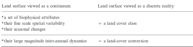
Table 2. Discrete versus continuous representation of land cover and land-cover change.

Land surface viewed as a continuum: Land surface viewed as a discrete reality:

∗a set of biophysical attributes

∗their fine scale spatial variability =a land cover class

∗their seasonal changes

∗their large magnitude inter-annual dynamics =a land-cover conversion

resolution, for the region of the African Sahel was values of some of the biophysical attributes, for just part of the seasonal cycle would probably also enter produced by A. Sneessens, G. Schayes and E. F. Lambin

(in prep.) (Table 1). The IGBP-DIS land cover map in that category. In that case, there is, however, a fuzzy boundary between processes of land-cover modification was derived through a classification of remote sensing

data (Loveland & Belward, 1997). Each category and conversion.

This suggests that monitoring forest degradation by corresponds to a dominant vegetation type or a mosaic

of vegetation cover types. A study of the characteristics remote sensing requires the measurement of a set of indicators of the biophysical attributes of the surface, of each cover has allowed Sneessens, Schayes & Lambin

(in prep.) to derive from literature and field observation the seasonality of these attributes, and their fine-scale spatial pattern. These information requirements data the range of values taken by each category for a

number of biophysical variables that are discriminant correspond to the three different major information sources that can be provided by remote sensing. As between surface covers. Field campaigns such as

HAPEX-Sahel in Niger (Princeet al., 1995) provide a forest degradation usually occurs slowly through land-cover modifications (not conversions), improved strong empirical basis for relating land-cover categories

to a distribution of attribute values. understanding of this complex ecological process requires an integration of the spectral, spatial and The discrete representation of land cover has the

advantages of concision and clarity, and represents a temporal information domains of remotely sensed data. low data volume. It is, however, a highly abstract model

of real landscapes. In the continuous representation of land cover, the biophysical variables vary continuously,

not only in space but also in time, at the seasonal

_{SPECTRAL, SPATIAL AND}

and inter-annual scales. By contrast, in the discrete

_{TEMPORAL INFORMATION ON}

representation of land cover, each spatial unit is

_{FOREST DEGRADATION}

represented by a single categorical value that is stable over a season (Table 2). Inter-annual changes in the

Spectral information

values of the biophysical attributes of the surface are

described as land-cover conversions only if the changes The estimation by remote sensing of biophysical attributes that are indicative of forest degradation has exceed the range of values that is characteristic of the

land-cover category (i.e. if the magnitude of the change been conducted using either an empirical approach or a physically-based approach. In the empirical approach, is such that the values of all biophysical attributes fall

within the range of another land cover class during the many authors have characterized the surface using vegetation indices that are arithmetic combinations of entire seasonal cycle). A land-cover modification—

which is not detectable with the discrete representation spectral bands. Most of these indices are variants of the normalized difference vegetation index (NDVI), of land cover—implies that variations in the values of

the biophysical attributes remain within the range of computed as the ratio between the difference and the sum of the radiances measured in the near infra-red values that is characteristic of the land-cover category.

Processes that lead to changes in the seasonal dynamics and red parts of the electromagnetic spectrum. These variants display different levels of sensitivity to or in the fine scale spatial variability of biophysical

Eric F. Lambin

Empirical studies and simulations with radiative more comprehensively surface processes for land-cover change studies (Lambin & Ehrlich, 1996, 1997; Nemani transfer models support the interpretation of vegetation

indices in terms of the fraction of photosynthetically et al., 1996). The slope of theTs-NDVIrelationship is interpreted in terms of surface resistance to active radiation absorbed by the vegetation canopy,

canopy attributes (e.g. green biomass or green leaf area evapotranspiration (Nemani & Running, 1989). At a finer spatial resolution, Pickup, Chewings & index), state of the vegetation (i.e. vegetation vigour

or stress) and instantaneous rates associated with the Nelson (1993) successfully tested a specific combination of spectral bands to monitor changes in vegetation activity of the vegetation (Myneniet al., 1995).

Inter-annual variations in primary production in the Sahel cover and to identify processes of land degradation in arid rangelands. Their empirical index provided a have been monitored using annual integration of

vegetation index data at a coarse spatial resolution good estimate of cover from remote sensing data, and included a standardization for multi-temporal data. (Hellden, 1991; Tucker et al., 1991). Similar data

have also been used to detect large-scale tropical This study suggested that the best characterization of the vegetation cover may be obtained with a different deforestation (Tucker, Holben & Goff, 1984; Woodwell

et al., 1987). The methods used in these studies are index for different ecosystems.

Physically-based approaches, relying on model not necessarily suitable for the detection of changes

associated with slow rates of land degradation due to inversion, have also been developed (e.g. Goel & Strebel, 1983; Li & Strahler, 1986; Pinty & Verstraete, spatial and temporal sampling issues. First, the level

of spatial aggregation of the data used in these studies 1992; Gobronet al., 1997). In these methods, a scene model is constructed to describe the form and nature (i.e. 8 by 8 km in the case of pre-processed time series

of Global Area Coverage data from the Advanced of the energy and matter within the scene and their spatial and temporal order (Strahler, Woodcock & Very-High Resolution Radiometer on the NOAA series

of orbiting platforms) is too coarse to allow for the Smith, 1986). This scene model is coupled with an atmospheric and a sensor model. This coupled remote detection of subtle changes in the density or structure of

vegetation cover. Second, integrating vegetation index sensing model is then inverted to infer, from the remotely sensed measurements, some of the properties data on an annual basis hides variations in the

phenological cycle of the vegetation cover. Third, the or parameters of the scene that were unknown (Strahler, Woodcock & Smith, 1986). Concerning tropical forest time consistency of the data over several years is not

always ensured due to, in the case of AVHRR, a ecosystems, these methods are not yet sufficiently robust to be applied routinely for a large-scale lack of on-board calibration of radiances, instrument

change-over, and a drift in equator crossing-time of monitoring of forest-cover changes, due to the difficulty for representing adequately in a model the natural the satellite’s orbit over the years. Time series of high

spatial resolution data can overcome several of these variability in landscape structure and composition. For example, Franklin & Strahler (1988) applied a limitations.

Land surface temperature (Ts), derived from the model inversion approach to generate regional estimates of tree size and density in West Africa, using thermal channels of satellite sensors, has also been used

as a biophysical indicator of the surface in empirical Landsat TM data. They used the Li-Strahler canopy reflectance model (Li & Strahler, 1986). A woodland studies.Tsis related, through the surface energy balance

equation, to surface moisture availability and evapo- stand is modelled geometrically as a group of objects casting shadow on the background. The reflectance of transpiration, as a function of latent heat flux (Carlson,

Perry & Schmugge, 1990). A few empirical studies have a pixel is modelled as a linear combination of the signatures of the major scene components (i.e. demonstrated the potential of these data for

land-cover change analysis, e.g. to detect forest disturbances illuminated tree crown, illuminated background, shadowed tree and shadowed background), weighted (Tuckeret al., 1984; Estreguil & Lambin, 1996), to

locate the boundary between shrub and woodland by their relative areas. Inversion results over a sample of observations were satisfactory for the estimation of savannas in West Africa (Malingreau, Tucker &

Laporte, 1989), or to map the boundary between tree density and cover but poor for tree size. The application of this type of approach for monitoring tropical rain forest and savanna vegetation (Achard &

Blasco, 1990). A few authors have combined a woodland degradation would probably require further developments for a more robust approach.

Remote sensing of forest degradation

Spatial information

improved when using both spectral (e.g. vegetation index and surface temperature) and spatial indicators A major attribute of a landscape is its spatial pattern.

of surface condition. Their study suggested that the The concept of landscape spatial pattern covers, for

detection of inter-annual changes in landscape spatial example, the patch size distribution of residual forests,

structure is more likely to reveal long term and long the location of agricultural plots in relation to natural

lasting land-cover changes while spectral indicators are vegetation, the shapes of fields and the number, types

more sensitive to fluctuations in primary productivity and configuration of landscape elements. Landscape

associated with the inter-annual variability in climatic spatial pattern is seldom static due both to natural

conditions. The long term monitoring of landscape changes in vegetation and to human intervention. The _{spatial pattern in addition to other biophysical} spatial dynamics of landscapes interact with ecological

variables can thus lead to the detection of a greater processes that have important spatial components _{range of processes of landscape modification (Lambin} (Turner, 1989), e.g. flows of energy, and matter between

& Strahler, 1994).

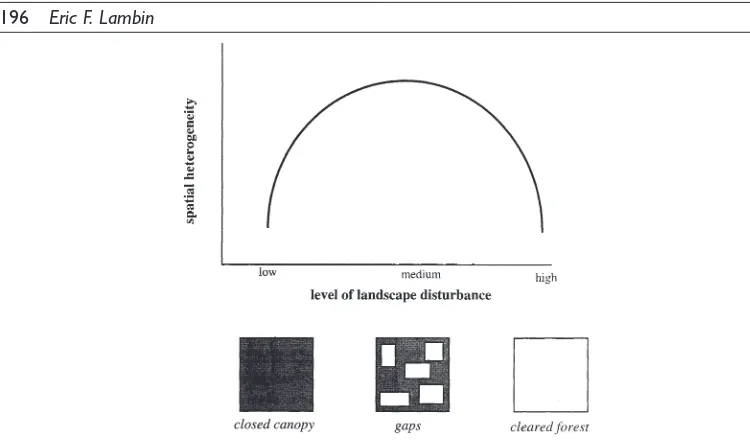
landscape elements, biological productivity of different _{The spatial pattern of a changing landscape also} components of the ecosystem, biodiversity, and the _{contains some information on the processes of} land-spread of disturbances. _{cover change. Certain categories of changes in human} Remote sensing offers the possibility to analyse _{land use tend to fragment the landscape (e.g. expansion} changes in spatial structure at the scale of landscapes _{of extensive agricultural exploitation, forest} degrada-(e.g. Briggs & Nellis, 1991; Dunnet al., 1991; Turner _{tion driven by small-scale logging, overgrazing or} & Gardner, 1991). Indicators of the degradation of the _{desertification around deep wells). Other land use} vegetation cover can be derived from such measures _{changes increase landscape homogeneity (e.g.} large-(Jupp, Walker & Pendridge, 1986; De Pietri, 1995). _{scale intensive cultivation or ranching). Spatial} For example, Pickup & Foran (1987) developed a _{processes of gap expansion in a forest cover have been} method to monitor arid landscapes used for pastoralism _{modelled to predict the total gap area and gap size} based on the spatial variability of the vegetation. The _{distribution (Kubo, Iwasa & Furumoto, 1996). One} spatial autocorrelation function and mean-variance _{can hypothesize that landscapes with a very low or} plots of a spectral indicator were found to be successful _{very high level of disturbance are characterized by} in discriminating between the cover responses typical _{a low spatial heterogeneity, while landscapes with a} of good and poor rainfall years. For drought _{medium level of disturbance are very heterogeneous.} conditions, the decrease in spatial autocorrelation with _{This would lead to the relationship sketched in Fig. 1.} increasing spatial lag was rapid since the ground surface _{Recent remote sensing observations generally support} is bare and most of the vegetation signal comes from _{this hypothesis, e.g. in a study of forest-cover} scattered areas of trees and shrubs. A low decay rate _{disturbances in Papua New Guinea (Estreguil &} of the autocorrelation function indicated a greater _{Lambin, 1996) and another study of forest} spatial uniformity of the landscape, e.g. during wet _{fragmentation in New England (Vogelmann, 1995).} periods, when more ground cover is present so reducing _{However, the validity of this model is likely to depend} the contrast between the bare soil signal and that on the scale of analysis. It is only when the spatial produced by trees and shrubs (Pickup & Foran, 1987). _{scale of observation of the landscape pattern is slightly} Similar observations were made by Lambin (1996) broader than the spatial scale of the impacts on over the seasonal and inter-annual cycle of three West _{landscape of a given disturbance that this inverted ‘U’} African landscapes. Vogt (1992) also analysed the shape is likely to be observed.

seasonal changes in spatial structure of a West African landscape, showing that there is a marked seasonal

Temporal information

cycle in the spatial structure of a vegetation index

Eric F. Lambin

Fig. 1. Sketch of the expected relationship between the level of landscape disturbance and the spatial heterogeneity of the landscape measured on spatial data at a spatial resolution of a few dozens of metres.

the vegetation cover. The analysis of the temporal shifts in the timing of rains and episodic events to which most ecosystems display a high resilience. In a trajectories of vegetation indices based on high

temporal frequency remote sensing data allows us to study that opens a new line of research, Goward & Prince (1995) provided empirical data, measured by monitor vegetation phenology and biome seasonality

(Justiceet al., 1985). remote sensing, that indicate some persistence or lag between vegetation activity and climate dynamics. In Processes such as a shortening of the growing season,

a dephasing of the phenology of different vegetation some ecosystems, the response time of vegetation to short-term climatic fluctuations might provide useful layers, or modifications of the cover due to disturbances

such as fires, can only be detected if inter-annual information on the level of forest degradation. Actually, changes in species composition affect the resilience of changes in the seasonal trajectories of vegetation covers

are analysed. For any landscape with a strong seasonal a given vegetation cover as different communities of trees, shrubs and grasses are characterized by di_fferent signal, the detection of inter-annual changes needs to

take into account explicitly the fine-scale temporal phenological growth response rates.

In addition to the monitoring of remotely sensed variations. If data from only one or a few dates a

year are used to measure inter-annual changes, the indicators of forest degradation, one can integrate a monitoring of its proximate causes or of other surface undersampling of the temporal series hinders the

change detection accuracy and might lead to the processes closely associated with the state of the vegetation cover. The best example of such a process detection of spurious changes (Lambin, 1996).

A quantitative evaluation of differences in seasonal for tropical ecosystems is biomass burning. Recent research has improved the ability to monitor active development curves of remotely sensed data was

applied for land-cover change analysis by Lambin & fires and burnt areas by remote sensing (Justiceet al., 1996; Eva & Lambin, 1998). On one hand, open forest Ehrlich (1997). In this study, a measure of the deviation

in seasonal trajectories was computed for 10 years of degradation may result from repeated biomass burning or be caused by a change in the fire regime. On the continental-scale remote sensing data. Subtle processes

of land-cover change could be detected this way. Results other hand, ecosystem degradation is likely to lead to a modification of the seasonal distribution and spatial suggested that land-cover changes in Africa mostly

involve erratic variations in land-cover conditions due patterning of fires as the diffusion of fires through the landscape will be altered.

Remote sensing of forest degradation

measure using remote sensing.Photogram. Eng. Remote

CONCLUSION

Sens.57, 407–411.

Carlson, T.N., Perry, E.M. & Schmugge, T.J. (1990) Some important lessons may be learnt from this review.

Remote estimation of soil moisture availability and (i) Degradation of forest-cover is often a complex _{fractional vegetation cover over patchy vegetation.} process, with some degree of reversibility as the _{Agric. Forest Meteorol.52, 44–60.}

biological productivity of forests is partially controlled Coppin P.R. & Bauer M.E. (1996) Digital change detection in forest ecosystems with remote sensing imagery. by climatic fluctuations. (ii) Only a representation of

Remote Sensing Rev.13, 207–234. land cover as a continuous field of several biophysical

DeFries, R.S., Field, C.B., Fung, I., Justice, C.O., Los, S., variables can lead to an accurate detection of forest

Matson, P.A., Matthews, E., Mooney, H.A., Potter, degradation. (iii) Repetitive measurements of spectral,

C.S., Prentice, K., Sellers, P.J., Townshend, J.R.G., spatial and temporal indicators of the land surface _{Tucker, C.J., Ustin, S.L., Vitousek, P.M. (1995) Mapping} have to be performed. (iv) Each set of indicators brings the land surface for global atmosphere-biosphere models: toward continuous distributions of vegetation’s a specific form of information on the land cover. These

functional properties.J. Geophys. Res.100 (D10), 20, indicators must therefore be combined to achieve a

867–20,882. comprehensive description of the surface processes. (v)

De Pietri, D.E. (1995) The spatial configuration of A long time series of observations is required to be

vegetation as an indicator of landscape degradation due able to detect trends in forest degradation that depart _{to livestock enterprises in Argentina.J. Appl. Ecol.32,} in a significant way from short-term, climate-driven 857–865.

Dunn, C.P., Sharpe, D.M., Guntenspergen, G.R., Stearns, fluctuations in forest conditions. Finally, (vi) a

F. & Yang, Z. (1991) Methods of analyzing temporal monitoring system can combine indicators of the

changes in landscape pattern. Quantitative methods in degradation itself, its proximate causes, and other

landscape ecology. The analysis and interpretation of surface processes linked with the vegetation cover.

landscape heterogeneity(ed. by M. G. Turner and R. H. One of the key implications of this review is the _{Gardner), pp. 173–198. Springer-Verlag, New York.} requirement for an integration of information from the Estreguil, C. & Lambin, E. (1996) Mapping forest spectral, spatial and temporal domains to monitor disturbances in Papua New Guinea with AVHRR data.

J. Biogeogr.23, 757–773. forest degradation. The main mechanisms for achieving

Eva, H. & Lambin, E.F. (1998) Remote sensing of biomass this are: (i) construction of empirical indices, i.e.

burning in tropical regions: sampling issues and mathematical formulations combining metrics from

multisensor approach. Remote Sens. Environ. 64, different information sources; (ii) multi-criteria _292–315.

analyses of forest degradation, either using statistical _{Franklin, J. & Strahler, A.H. (1988) Invertible canopy} classification methods or a set of knowledge rules; or reflectance modeling of vegetation structure in semiarid woodland.IEEE Trans. Geosci. Remote Sensing,

GE-(iii) development of invertible remote sensing models

26, 809–825. that represent key variables related to the level of

Gobron, N., Pinty, B., Verstraete, M.M. & Govaerts, Y. degradation of forest covers. All three approaches need

(1997) A semi-discrete model for the scattering of light to be calibrated against a statistical sample of field

by vegetation.J. Geophys. Res.102, 9431–9446. observations of biophysical attributes that characterize _{Goel, N.S. & Strebel, D.E. (1983) Inversion of vegetation} forest conditions. As different monitoring systems may canopy reflectance models for estimating agronomic variables. i. Problem definition and initial results using be optimal for different ecosystems, this calibration

Suits model.Remote Sens. Environ.13, 487–507. should probably be done at the level of ecosystems.

Goward, S.N. & Prince, S.D. (1995) Transient effects of We still need to accumulate case studies to identify

climate on vegetation dynamics: satellite observations. which approach and which combination of information

J. Biogeogr.22, 549–563.

sources works best for different ecosystems. _{Grainger, A. (1993)Controlling tropical deforestation, p.}

310. Earthscan Publications Ltd, London.

Hellden, U. (1991) Desertification—Time for an

REFERENCES

Assessment?Ambio,20, 372–383.

Jupp, D.L.B., Walker, J. & Pendridge, L.K. (1986) Interpretation of vegetation structure in Landsat MSS Achard, F. & Blasco, F. (1990) Analysis of vegetation

imagery: a case study in disturbed semi-arid eucalypt seasonal evolution and mapping of forest cover in West

woodland. Part 2. Model-based analysis. J. Environ. Africa with the use of NOAA AVHRR HRPT data.

Mgmnt.23, 35–57. Photogram. Eng. Remote Sens.56, 1359–1365.

Justice, C.O., Kendall, J., Dowty, P. & Scholes, R.J. (1996) Briggs, J.M. & Nellis, J.M. (1991) Seasonal variation

Eric F. Lambin

campaign using NOAA advanced very high resolution Pinty, B. & Verstraete, M.M. (1992) On the design and validation of surface bidirectional reflectance and albedo radiometer data. J. Geophys. Res. 101 (D19), 23,

851–863. models.Remote Sens. Environ.41, 155–167.

Prince, S.D., Kerr, Y.H., Goutorbe, J.-P., Lebel, T., Tinga, Justice, C.O., Townshend, J.R., Holben, B.N. & Tucker,

C.J. (1985) Analysis of the phenology of global A., Bessemoulin, P., Brouwer, J., Dolman, A.J., Engman, E.T., Gash, J.H.C., Hoepffner, M., Kabat, P., Monteny, vegetation using meteorological satellite data. Int. J.

Remote Sens.6, 1271–1318. B., Said, F., Sellers, P. & Wallace, J. (1995) Geographical, biological and remote sensing aspects of the Hydrologic Kubo, T., Iwasa, Y. & Furumoto, N. (1996) Forest spatial

dynamics with gap expansion: total gap area and gap Atmospheric Pilot Experiment in the Sahel (HAPEX-Sahel).Remote Sens. Environ.51, 1.

size distribution.J. Theor. Biol.180, 229–246.

Lambin, E.F. (1996) Change detection at multiple temporal Prins, E. & Kikula, I.S. (1996) Deforestation and regrowth phenology in Miombo woodland assessed by Landsat scales: seasonal and annual variations in landscape

variables.Photogram. Eng. Remote Sens.62, 931–938. Multispectral Scanner System data.Forest Ecol. Mgmnt.

84, 263–266. Lambin, E.F. & Ehrlich, D. (1996) The surface

temperature-vegetation index space for land cover and Ringrose, S., Matheson, W., Tempest, F. & Boyle, T. (1990) The development and causes of range degradation land-cover change analysis.Int. J. Remote Sensing,17,

463–487. features in southeast Botswana using multi-temporal Landsat MSS imagery.Photogram. Eng. Remote Sens. Lambin, E.F. & Ehrlich, D. (1997) Land-cover changes in

sub-Saharan Africa (1982–1991): Application of a 56, 1253–1262.

Strahler, A.H., Woodcock, C.E. & Smith, J.A. (1986) On change index based on remotely-sensed surface

temperature and vegetation indices at a continental scale. the nature of models in remote sensing.Remote Sens. Environ.20, 121–139.

Remote Sens. Environ.61, 181–200.

Lambin, E.F. & Strahler, A.H. (1994) Indicators of land- Tucker, C.J., Dregne, H.E. & Newcomb, W.W. (1991) Expansion and contraction of the Sahara desert from cover change for change-vector analysis in

multitemporal space at coarse spatial scales. Int. J. 1980 to 1990.Science,253, 299–301.

Tucker, C.J., Holben, B.N. & Goff, T.E. (1984) Intensive Remote Sensing,15, 2099–2119.

Li, X. & Strahler, A.H. (1986) Geometric-optical forest clearing in Rondonia, Brazil, as detected by satellite remote sensing. Remote Sens. Environ. 15, bidirectional reflectance modeling of a conifer forest

canopy.IEEE Trans. Geosci. Remote Sensing,GE-24, 255–261.

Turner, M.G. (1989) Landscape ecology: the effect of 906–919.

Loveland, T.R. & Belward, A.S. (1997) The IGBP-DIS pattern on process.Annu. Rev. Ecol. Syst.20, 171–197. Turner, M.G. & Gardner, R.H. (1991)Quantitative methods global 1 km land cover data set, DISCover: first results.

Int. J. Remote Sensing18, 3289–3295. in landscape ecology. The analysis and interpretation of landscape heterogeneity, Springer-Verlag, New York. Malingreau, J.P., Tucker, C.J. & Laporte, N. (1989)

AVHRR for monitoring global tropical deforestation. Turner, II B.L., Moss, R.H. & Skole, D.L. (1993)Relating land use and global land-cover change: a proposal for an Int. J. Remote Sensing10, 855–867.

Myneni, R.B., Maggion, S., Iaquinta, J., Privette, J.L., IGBP-HDP core project. IGBP Report no. 24, HDP Report no. 5, International Geosphere-Biosphere Gobron, N., Pinty, B., Kimes, D., Verstraete, M. &

Williams, D. (1995) Optical remote sensing of vegetation: Programme, Stockholm.

Verstraete, M.M. & Pinty, B. (1996) Designing optimal modelling, caveats and algorithms. Remote Sens.

Environ.51, 169–188. spectral indexes for remote sensing applications.IEEE Trans. Geosci. Remote Sensing,GE-34, 1254–1265. Nemani, R.R. & Running, S.W. (1989) Estimation of

regional resistance to evapotranspiration from NDVI Vogelmann, J.E. (1995) Assessment of forest fragmentation in southern New England using remote sensing and and Thermal-IR AVHRR data.J. Applied Meteor.28,

276–284. geographic information systems technology. Conserv. Biol.9, 439–449.

Nemani, R.R., Running, S.W., Pielke, R.A. & Chase, T.N.

(1996) Global vegetation cover changes from coarse Vogt, J. (1992) Characterizing the spatio-temporal variability of surface parameters from NOAA-AVHRR resolution satellite data. J. Geophys. Res. 101 (D3),

7157–7162. data, p. 266. Report EUR 14637 EN, Agriculture Series, Joint Research Centre, Institute for Remote Sensing Pickup, G., Chewings, V.H. & Nelson, D.J. (1993)

Estimating changes in vegetation cover over time in Applications, Italy.

Woodwell, G.M., Houghton, R.A., Stone, T.A., Nelson, arid rangelands using Landsat MSS data.Remote Sens.

Environ.43, 243–263. R.F. & Kovalick, W. (1987) Deforestation in the tropics: new measurements in the Amazon basin using Landsat Pickup, G. & Foran, B.D. (1987) The use of spectral and

spatial variability to monitor cover change on inert and NOAA AVHRR imagery.J. Geophys Res.92 (D2), 2157–2163.