Full Terms & Conditions of access and use can be found at
http://www.tandfonline.com/action/journalInformation?journalCode=ubes20
Download by: [Universitas Maritim Raja Ali Haji] Date: 12 January 2016, At: 23:35
Journal of Business & Economic Statistics
ISSN: 0735-0015 (Print) 1537-2707 (Online) Journal homepage: http://www.tandfonline.com/loi/ubes20
Contrasts Between Types of Assets in Fixed
Investment Equations as a Way of Testing Real
Options Theory
Ciaran Driver, Paul Temple & Giovanni Urga
To cite this article: Ciaran Driver, Paul Temple & Giovanni Urga (2006) Contrasts Between Types of Assets in Fixed Investment Equations as a Way of Testing Real Options Theory, Journal of Business & Economic Statistics, 24:4, 432-443, DOI: 10.1198/073500106000000062
To link to this article: http://dx.doi.org/10.1198/073500106000000062
Published online: 01 Jan 2012.
Submit your article to this journal
Article views: 61
View related articles
Contrasts Between Types of Assets in Fixed
Investment Equations as a Way of Testing
Real Options Theory
Ciaran DRIVER
Tanaka Business School, Imperial College, University of London, London SW7 2AZ, U.K. (c.driver@imperial.ac.uk)
Paul TEMPLE
Department of Economics, University of Surrey, Guildford GU2 7XH, U.K. (p.temple@surrey.ac.uk)
Giovanni URGA
Faculty of Finance, Centre for Econometric Analysis, Cass Business School, London EC1Y 8TZ, U.K. (g.urga@city.ac.uk)
This article tests the power of real options theory to explain investment under uncertainty, exploiting dif-ferences in the degrees of irreversibility and expandability between machinery and buildings. It reports estimates of investment equations for each asset class using a large sample of U.K. manufacturing in-dustries, with results that are consistent with the predictions of real options theory. In addition, using a specially constructed industry-specific measure of irreversibility for machinery investment, the article provides further confirmation of the empirical relevance of real options.
KEY WORDS: Investment; Irreversibility; Panel data; Real options; Uncertainty.
1. INTRODUCTION
Few topics in economics have generated such a vast literature as investment under uncertainty; however, it has proven very difficult to use the burgeoning theory in a way that imposes or-der on the applied results. It is easy to show that uncertainty can reduce the incentive to invest. If the firm can wait without severe penalties, and if committing now involves sunk costs, then there is clearly an advantage to waiting that reduces the in-centive to current investment. However, this conclusion can be reversed where costs are not sunk (i.e., there is a put option) or where waiting involves a penalty, as in the case of a firm being unable to respond to a future favorable shock because of some binding constraint (e.g., with respect to input supplies). In such cases the firm may be said to lack a call option that otherwise could be exercised by, for example, the purchase of inputs at a prearranged option price. Therefore, it is the overall balance of effects arising from both the put option and the call option that will determine the sign of the influence of uncertainty.
Our intention in this article is to test the predictions of real options theory by discriminating between the cases in which irreversibility (the lack of a put option) or expandability (the presence of a call option) matter most. We argue that there are important differences in this regard between broad classes of assets—machinery and buildings—that have implications for the effect of uncertainty on investment in each asset type. To an-ticipate our results, we find that machinery investment is more influenced downward and less influenced upward by uncer-tainty than building investment. The preponderance of negative results in the literature may reflect the weight of studies that es-timate machinery investment equations or aggregate equations that are dominated by the machinery component.
The article is organized as follows. The next section reviews the evidence for maintaining a distinction between the char-acteristics of our two asset types. Section 3 outlines the real
options approach and provides hypotheses that contrast build-ing and machinery investment under option theory. Section 4 specifies an investment equation, and Section 5 interprets and discusses the results of a set of investment equations for both classes of capital goods using seemingly unrelated regression estimation (SURE) and panel estimation. Section 6 expands the analysis by using a specially constructed industry-specific in-dex of irreversibility for machinery, which allows us to check for interaction effects between irreversibility and uncertainty for this class of investment. Section 7 concludes.
2. CONTRASTING ASSET TYPES
In this section we present evidence that our chosen two assets—machinery and buildings—are characterized by differ-ences in their respective levels of both irreversibility (sunk cost) and expandability. In the empirical literature, sunk cost has been estimated at an industry level from data on the minimum ef-ficient scale for new entry and auxiliary indicators, such as the extent of rental markets, depreciation rates, and the exis-tence of second-hand markets (Sutton 1991; Worthington 1995; Kessides 1990a; Ghosal 2002). In this article we are more con-cerned with assigning an irreversibility classification to differ-entassetsrather than to differentindustries, although we also consider variation by industry in Section 6.
What is the evidence that machinery investment is more irre-versible than buildings? It is often thought that markets for gen-eral machinery are frictionless, given that assets can be disposed of through organized second-hand sellers, not only at auctions.
© 2006 American Statistical Association Journal of Business & Economic Statistics October 2006, Vol. 24, No. 4 DOI 10.1198/073500106000000062
432
Driver, Temple, and Urga: Testing Real Options Theory 433
Indeed, some classic references in the literature (e.g., Hulten and Wykoff 1981) assume the existence of perfect second-hand markets to ascertain the depreciation pattern of specific classes of machinery. However, recent research has emphasized just how imperfect such markets are, due to the industry-specific nature of the assets and to thin-market effects. One study, based on an examination of equipment disposals after the closure of U.S. aerospace plants in the 1990s, found substantial industry specificity, a large discount relative to replacement cost, and a lengthy selling time (Ramey and Shapiro 2001). A similar study of the Swedish metal working industry (but concerned with rou-tine decisions rather than with those linked to a major sell-off ) found that the sunk cost component varied between 50% and 80% of the replacement cost; a majority of items—many com-paratively new—were scrapped at a negligible price rather than being sold (Asplund 2000). This suggests both industry- and firm-specificity. Note, moreover, that our data on machinery as-sets also include investment in process plants, which again is likely to be highly specific to its industry.
Turning now to buildings assets, it seems unlikely that the physical specifications are likely to change much between firms in the same narrow industry, implying that less firm specificity is involved than for machinery. There also may be less indus-trial specificity, given that buildings can be easily adapted for different purposes and frequently are. This question was in-vestigated by Worthington (1995), who used the proportion of rental payments in capital costs and the proportion of capital expenditure on used assets as inverse proxies for irreversibility. Computing these measures separately for equipment and struc-tures indicates that “equipment expendistruc-tures are more ‘sunk’ than structures. . .” (p. 59).
Additional evidence that buildings are less specific in use comes from a unique series of official data on gross increases and decreases in industrial floor space over the period 1982– 1985 for England (Government Statistical Service 1986). The data show that approximately 40% of the gross increase was due to a change to industrial use from other categories of floor space (warehouses, shops, restaurants, and commercial offices). The corresponding data on gross decreases in industrial floor space during the same period show that demolitions accounted for only one-quarter of the decline. In the United States, Ramey and Shapiro (2001) found that no buildings were sold in the aerospace closures studied. The authors explained this by the observation that “not selling buildings is not unusual for plant closings that are more than 25 years old. . .[Due to environmen-tal costs] they simply raze the buildings to the ground” (p. 965). Our results suggest that demolition is not as common as this, perhaps because many industries have less dedicated buildings than aerospace or because of greater pressure on land use in the densely populated U.K. The frequent change in use in both directions suggests that building assets are neither highly firm-specific nor even highly sector-firm-specific in most cases. Indeed, using the previously cited data source on U.K. floor space, we can compare the demolition ratio of industrial floor space with that for commercial offices and for shops and restaurants. The ratios are .24, .24, and .28, suggesting that the three categories are similar with respect to the decision to sell or scrap. This sup-ports the view that industrial buildings are not highly specific, because it is widely recognized that the offices and shops are
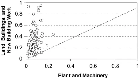
Figure 1. Ratios of Disposals to Acquisitions by Asset Class. Indus-tries with ratios>1 have been excluded.
fungible categories of assets in the sense of being easy to adapt for use by other owners.
Further evidence on the relative irreversibility of buildings versus machinery is provided by data on second-hand sales. The annual U.K. Census of Production contains current val-ues by three-digit industry of both disposals (the sale for any purpose of second-hand buildings and industrial land, as well as plant and machinery) and acquisitions (which may be either new or second hand). We use these data to construct a time-averaged ratio (1979–1989) of disposals to acquisitions for the two classes of assets: machinery and buildings, where the build-ings category includes industrial land. This is plotted in Fig-ure 1, which shows that the ratio is nearly always substantially higher for the land and buildings category than for machinery. This again supports the argument that sunk costs are higher for machinery.
In further support of this dichotomy between machinery and building assets, there is at least one piece of indirect evidence arising from work on entry barriers. Kessides (1990b) showed that machinery investment is more effective than building in impeding entry. This is even after taking account of the profit level of incumbents, the growth of industry demand, and the required scale of entry. Quite plausibly, this is because the sunk component of the former is greater. Indeed, the finding is that although industry variation in the upper bound of sunk cost for machinery and equipment exerts a significant negative effect on entry, the corresponding buildings variable has no significance. The preceding discussion has demonstrated that machinery is characterized by greater irreversibility than buildings. It also seems highly likely (although admittedly there is less evidence to cite) that building assets display less expandability than machinery. This is first because machinery purchases are less lumpy than buildings and often can be bought from stock in any number without long delivery lags. In contrast, building al-terations and expansions require design, planning approval, and site availability, and expandability may not even be feasible in some circumstances. A further point of contrast concerns the cyclicality of supply price for the two assets. The U.K. building deflator is highly cyclical due to labor intensity and a reliance on heavy materials, such as bricks and cement, that have high transport costs. Firms that fail to add sufficient capacity at the right time can expect to pay a high premium if they have to bid for expansion as demand strengthens. Using Office of Na-tional Statistics data, the ratio of the annual variance of the real
price of machinery to the corresponding variance for buildings is<.4 for a 30-year period that spans our dataset. Accordingly, we expect expandability to be greater for the machinery class of assets.
3. INVESTMENT THEORY AND REAL OPTIONS
Until quite recently, investment theory has been dominated by models of continuous adjustment implied by the convex cost of adjustment approach. Such models have typically been solved using stock market valuation for the marginal value of a unit of capital, by representing that marginal value by a vector autoregression, or by invoking rational expectations
for the value of marginal q. However, such standard models
have tended to disappoint in empirical estimation (Chatelain and Teurlai 2001; Driver and Meade 2001).
Recently, a class of models has been proposed that focuses on potential discontinuities in the adjustment process (Caballero 1999). Much of this literature focuses on the “irreversibility
pre-mium” or the multiple by which Tobin’sqmust be adjusted to
take into account the absence of a put option when investing (Dixit and Pindyck 1994, p. 146). However, it is not clear that the premium is always positive; indeed, we may talk of an “ex-pandability” premium when the former is negative. This com-plication is identified in the contribution of Abel, Dixit, Eberly, and Pindyck (1996). In a two-period investment model, the ex ante investment may no longer be appropriate in the light of the realization of the stochastic variablee[see (1)]. In the second period, one might prefer to sell part of the capital invested or exercise a right to buy more at a prearranged price. Here the ex post price for a disequilibrium adjustment,whether up or down, is distinguished from the ex ante purchase price. This compli-cation results in a premium to be discounted and added to the Jorgenson user cost of capital term (Abel et al. 1996, expres-sion 17),
of capital and the corresponding (ex post) selling and buying prices. The first and third terms reflect the fact that not only ex-cess capital may have to be disposed of at a distress price (p−),
but also deficient capital may need to be installed at a premium price (p+). The middle (integral) term reflects the expected
di-vergence between price and marginal return, where the discrep-ancy is not sufficient to induce contraction or expansion.F(e)is the distribution function of the underlying stochastic variable, andRK is the marginal return on capital installed, which may
have to be evaluated at a nonoptimal level of the capital stock. The terms eL andeH are the critical values of the stochastic
variable at which the original capital is no longer optimal ex post, which signal the need to adjust the capital stock at a dise-quilibrium price. The effect of this modification is to show the possibility of an irreversibility option premium or an expand-ability option premium (i.e., the hurdle rate can lie above or be-low the usual cost of capital). The irreversibility premium will exist where deferral options effects are dominant (i.e., the fear
of being locked into uneconomic commitments). The expand-ability premium will exist where the dominant concern is the ability to ensure capacity in the event of favorable demand.
To derive specific hypotheses, we note that the incentive to invest depends on the level of the two exercise prices,
p− and p+. This can be demonstrated by differentiating the
shadow value of capital (termedq, eqs. 6 and 7 in Abel et al.
1996) with respect to p− and p+. Because the only terms in
these variables are the terms(p−p−)F(eL)and−(p+−p)[1−
F(eH)], it is obvious that the marginal value of capital is
in-creasing in bothp−andp+. Intuitively, an increase in the resale
price (p−) reduces irreversibility and increases the incentive to
invest, whereas an increase in the contingent purchase pricep+
reduces the value of the call option and increases the marginal value of current investment (Abel et al. 1996, pp. 760–761).
Abel et al. (1996) derived the cumulative probability den-sity function (cdf ) of the marginal return to first-period capital
RK(K,e)as a function of the underlying distribution of e. As
noted earlier, it may be optimal to adjust the first-period capi-tal ex post; these exchanges are effected at the exercise prices
p−andp+. The expectation of first-period marginal returns to capital must take into account these ex post adjustments. Abel et al. (1996) plotted the cdf ofRK(K,e)with critical values
p−andp+cutting off areas corresponding to the values of the
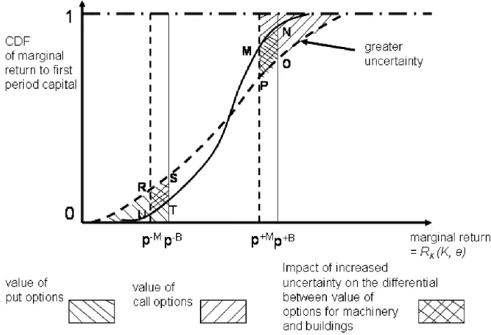
put and call options. We reproduce that plot in Figure 2 with the modification of showing two distributions corresponding to a mean-preserving spread in the outcome variableethat trans-lates into greater dispersion in the marginal return. The distri-bution with the higher dispersion has higher values ofbothput and call options; however, what is of interest in our analysis is how thedifferencesin option values behave as we shift atten-tion from one class of assets to another. We have argued earlier that machinery is characterized by a lowp− and lowp+ rela-tive to building; that is, there is both greater irreversibility and greater expandability for machinery. Therefore, in Figure 2 we also depict the distribution tails for both asset classes. A con-ceptual shift in the cutoff points from the full vertical lines to the dashed vertical lines corresponds to a shift from buildings to machinery.
The model of Abel et al. (1996) involves a generalization of Bernanke’s “bad news principle” (Bernanke 1983) in which a redistribution of probability mass within the upper tail of Fig-ure 2 leaves the shadow value of capital unaffected and thus is irrelevant to investment decisions. Bernanke considered only the upper tail of the distribution due to his twin assumptions of complete expandability of capital at a fixed rental and total irre-versibility so that disposal value is zero. Thus “good news” does not matter; that is, within the upper tail, even better news has no effect, because that part of the distribution is not operative. The more general model of Abel et al. produces a “good and bad news” principle, in which the redistribution of probability mass withineithertail has no effect onq, as the firm will sell capi-tal at the distress or floor price or buy capicapi-tal at the contingent price that has been contracted (partial expandability).
For any given project, the effect of increased uncertainty on the incentive to invest is thus ambiguously signed. Greater un-certainty tends to increase the weight of both tails; that is, the value of both the put option and the call option is increased. A higher put option value (with a larger left tail)—reflecting
Driver, Temple, and Urga: Testing Real Options Theory 435
Figure 2. Impact of an Increase in the Mean Preserving Spread (adapted from Abel et al. 1996).
the increased likelihood of exercising the opportunity to ad-just downward at the strike pricep−—increases the incentive to invest relative to the no option case, whereas a larger call option value (a larger right tail)—reflecting the increased like-lihood of exercising the opportunity to adjust upward ex post at thep+ strike price—reduces the incentive to invest relative
to the no option case. The net effect on investment of increased uncertainty is thus ambiguous, with a positive effect coming from the increased put option and a negative effect from the increased call option (Abel et al. 1996, p. 773; Bar-Ilan and Strange 1996).
However, thedifferentialeffect of increased uncertainty be-tween buildings and machinery is not ambiguous. As is clearly shown in Figure 2, greater uncertainty increases the call option value of machinery by a greater amount than the call option of buildings. In the figure, this difference is shown by the cross-hatched area MNOP. In contrast, greater uncertainty increases the put option of buildings by more than the put option of ma-chinery (with the difference here given by the cross-hatched area RSTU). This contrast opens up the possibility of an empir-ical test of real options theory, as outlined in the next section.
To set up a test that discriminates between the effect of un-certainty on our two asset classes, we first identify separate pan-els with positive and negative uncertainty effects. The negative signed cases will be dominated by the increased call option ef-fect. Focusing on this (the right tail), the effect of increased uncertainty is to increase the value of the call option,but to increase it more for machinery relative to buildings. Thus in-creased uncertainty will have a differential negative effect
be-tween the assets, with a more pronounced negative effect for machinery.
A similar analysis may be made of the panels with positive uncertainty effect, which will be dominated by the increased put option effect. Focusing now on the left tail, the effect of increased uncertainty is again to increase the value of the put optionbut to increase it more for buildings relative to machin-ery. Thus increased uncertainty will have a differential positive effect between the assets, with the positive effect being more pronounced for buildings. Note that we ignore the effect of con-vexity or concavity on the marginal return between the critical points, because there is no strong prior as to differences in this between the asset types.
We may summarize the predictions of the foregoing analysis in a simple matrix corresponding to the industry panels that we investigate herein. This is given Table 1.
4. MODEL SPECIFICATION
To test the existence of real options effects, we contrast in-vestment equations for both machinery and buildings for a set of U.K. industries. Given the difficulties in specifying and esti-mating Euler equation models (Garber and King 1983; Chirinko 1993), we have recourse to a standard flexible accelerator model that incorporates direct expectations and survey data from the main U.K. employers organization, the CBI. As other recent research has argued (e.g., Mairesse, Hall, and Mulkay 1999), these direct expectations have advantages over the inference of expectations required in the Euler equation approach, especially when used in an error-correction type model.
Table 1. Prediction of the Relative Magnitude of Uncertainty Coefficients for Four Panels
Machinery Building
Positive uncertainty coefficients panel Less positive than building More positive than machinery Negative uncertainty coefficients panel More negative than building Less negative than machinery
The survey data (which are publicly available and feed into the European Union industrial database) record investment au-thorization rather than actual investment, although these two variables are linked by a well-determined realization function (European Commission 1997; see also Lamont 2000 for the ac-curacy of U.S. intentions data). The data are qualitative, being recorded in the form of the percentage of respondents reply-ing “more” or “less” to the level of authorizations planned in the next period. However, a useful result is that the balance of “more” over “less” responses is closely correlated with rates of change (Driver and Urga 2004; Smith and McAleer 1995). The specification for the balance in investment authorizations (At) is
derived as an optimal response to adjustment costs (see Berndt 1990; Chirinko, Fazzari, and Meyer 1999). We include uncer-tainty variables along with a set of other relevant variables from the CBI survey (see App. A).
We specify a log-linear accelerator equation linking invest-ment authorizationsAtand change in outputYt,
logAt=α+βlogYt+εt.
Representing this in equilibrium-correction form, specified on the assumption thatAtandYtmay be nonstationary and
coin-tegrated with a cointegrating scalar of 1, we have
logAt=β0+β1logYt+β2log(A/Y)t−1+et, (2)
whereetis an iid error term.
The dependent variable and both of the terms involvingYt
were constructed as discussed earlier from the survey data balances of “ups” over “downs” with respect to responses to the authorization question and the output question. Therefore, these balances represent growth rateslogAtandlogYt, as
demonstrated in the literature on survey transformations. Thus the dependent variable may be directly read from the survey in-formation, but the terms inYtrequire further transformations
of the data as specified in Appendix A. The equilibrium error-correction term log(A/Y)t−1 represents the extent to which
authorized investment is tracking incremental output; integrat-ing these terms gives the ratio of authorized capital to output or, inversely, the capacity utilization term often used in investment equations to proxy an (integral control) equilibrium-correction term.
Thus the basic specification (the full derivation is reported in App. A) is a modified form of (2),
autht=b0+b1yt+b2cut−1+et, (3)
where the dependent variable(autht)is the balance of replies to
survey Question 3 used to proxylogAt; the variableyt is the
approximation to the second term in (2) derived in Appendix A from the survey data; andcut−1is the lagged capacity
utiliza-tion term also derived in the Appendix A from the survey data to proxy the third term in (2). Coefficientsb1andb2are both
expected to be positive.
Equation (3) can be directly estimated by the CBI survey data. To obtain the reduced form of the estimated equation, we further assume that investment authorization is affected by
its own lagged values(
jautht−j), by the degree of optimism
about the general business situation (optt), by a measure of financial constraints (fi), by the degree of uncertainty (unct),
and by the current value of the differenced log term in
capac-ity utilization (dlcut). Because the CBI survey contains two
kinds of information on output, the forward-looking term and the backward-looking term (see Question 8 in App. A), our model includes both forward and backward terms ofyt, denoted
byyftandybt. After experimentation, we include only the cur-rent value ofyftand both the current and lagged values ofybt
in our specification. The reduced form of the equation that we estimate throughout the article is
authit=bi,0+
The explanatory variable measuring industry-level business confidence or optimism (opt) is obtained from replies to Ques-tion 1 of the survey. Our uncertainty variable (unc) is based on the cross-sectional dispersion of beliefs across firms in an
industry with regard to optimism for theindustry. Assuming
a high degree of homogeneity in demand conditions within the industry, the cross-sectional dispersion of beliefs about the same sector may be considered a measure of uncertainty. This entropy variable has been used successfully in other contexts involving surveys with three possible replies to measure the extent of disagreement among respondents (Fuchs, Krueger, and Poterba 1998; Zarnowitz and Lambros 1987; Giordani and Soderland 2003; Lensink, Bo, and Sterker 2001). Herefiis the expected incidence of internal or external financial constraints as measured by the percentage giving either type as a reply to CBI Question 16c (see App. A).
5. EMPIRICAL RESULTS
First, we performed unrestricted (slope coefficients varying across equations) SURE, because in the presence of contempo-raneous correlation, it is more efficient to estimate all equations jointly rather than estimate each of them separately. Summary result statistics for each industry for both machinery and build-ings are given in Appendix B, which shows that the specifica-tion of the investment equaspecifica-tions is supported by the data for both machinery and buildings. The coefficients in the SURE equations are generally significant and signed in accordance with expectation with generally acceptable diagnostics. To bet-ter understand these results, we moved to a more parsimonious representation of the estimates by pooling across industries. Table 2 (columns 2 and 3) reports the preferred pooled mod-els (fixed effects for machinery, random effects for buildings), with the fixed effects for buildings also included for compar-ison in column 4. These results for the whole panel show an overall negative effect of uncertainty on machinery investment. For buildings, the effect is positive but not significant. However, using SURE to model the considerable heterogeneity across in-dustries in the buildings sample is further justified by the test of Breusch and Pagan (1980). The null that contemporaneous co-variances are 0 (see Judge, Hill, Griffiths, Lutkepohl, and Lee 1988, p. 455) is rejected, favoring unrestricted SURE (see Ta-ble 2).
The rejection of homogeneity in the total sample for build-ings suggests that it would be useful to split the samples when
Dr
iv
er
,
T
emple
,
and
Urga:
T
e
sting
R
eal
Options
Theor
y
437
Table 2. Panel Estimation: Dependent Variable: Investment Authorization
Machinery Buildings Buildings Machinery Machinery Buildings Buildings
Model Fixed effects Random effects Fixed effects Random effects Random effects Random effects Random effects
Sample Full Full Full Industries with
negative uncertainty term
Industries with positive uncertainty
term
Industries with negative uncertainty
term
Industries with positive uncertainty
term
Standardized Standardized Standardized Standardized Standardized Standardized Standardized coefficientsa coefficientsa coefficientsa coefficientsa coefficientsa coefficientsa coefficientsa
(t-values in (t-values in (t-values in (t-values in (t-values in (t-values in (t-values in parentheses)b parentheses)b parentheses)b parentheses)b parentheses)b parentheses)b parentheses)b
Explanatory variables
auth(−1) .28 .28 .26 .37 .21 .28 .17
(16.95)∗∗ (16.73)∗∗ (−15.22)∗∗ (8.40)∗∗ (3.74)∗∗ (8.66)∗∗ (2.88)∗∗
auth(−2) .16 .17 .15 .17 .05 .14 .12
(9.60)∗∗ (10.04)∗∗ (8.62)∗∗ (3.81)∗∗ (.98) (4.33)∗∗ (2.20)∗
opt .19 .15 .12 .21 .28 .16 .18
(9.58)∗∗ (6.93)∗∗ (6.94)∗∗ (4.09)∗∗ (3.97)∗∗ (3.72)∗∗ (2.39)∗
yf .05 .03 .02 .08 .08 .03 −.03
(3.33)∗∗ (2.08)∗ (1.92)+ (1.99)∗ (1.47) (−1.1) (−.44)
yb .07 .08 .04 .03 .06 .08 .01
(4.74)∗∗ (4.88)∗∗ (4.84)∗∗ (.73) (1.11) (2.60)∗∗ (.16)
yb1 .08 .06 .03 .09 .09 .12 .05
(5.21)∗∗ (3.82)∗∗ (3.83)∗∗ (2.21)∗ (1.71)+ (4.05)∗∗ −.82
cu1 .08 .06 3.55 .1 .11 .12 .18
(2.38)∗ (2.05)∗ (2.31)∗ (1.38) (.99) (2.03)∗ (1.52)+
unc −.04 −.00 −1.95 −.11 −.06
(−2.82)∗∗ (−.23) (−.04) (−3.18)∗∗ (−2.22)∗
unc(−1) −.01 −2.99 .08 −.09 .14
(−.42) (−.61) (1.64)+ (−3.26)∗∗ (2.66)∗∗
unc(−2) .02 4.0 −.08
(−1.12) (.81) (−2.06)∗
Sum ofuncsignificant
coefficients (pvalue) [0] [0]
fi(−1) −.01 −.02 .01 .04 .08 −.02 .01
(−.90) (−1.29) (−.12) −1.03 (1.86)+ (−.76) (−.22)
dlcu −.01 −.02 −.03 −.08 .02 −.10 −.08
(−.19) (−.67) (−1.05) (−1.15) (.23) (−1.82)+ (−.71)
constant −5.97 −19.96 −17.69 4.72 −23.21 −10.19 −43.73
(−1.24) (−4.46) (−3.67)∗∗ (.36) (−1.33) (−1.37) (−2.79)∗∗
No. of observations 3,516 3,515 3,515 546 378 1,014 378
R2 .49 .39 .37 .56 .58 .46 .49
Joint significance tests:
F-test (fixed-effects model) 36.98∗∗ 22.62∗∗
Wald test (χ2)
(random-effects model) 2,192.68∗∗ 580.47∗∗ 396.95∗∗ 685.05∗∗ 279.54∗∗
Hausman testc(pvalue) χ2(80)=108.7∗∗[.01] χ2(83)=63.67[.9] χ2(81)=6.97[1.0] χ2(83)= 7.84[1.0] χ2(84)=33.49[1.0] χ2(83)=3.08[1.0] Breusch–Pagan testd(pvalue) χ2(861)= 904.01[.15] χ2(861)=1,015∗∗[0] χ2(21)=37.91∗[.01] χ2(10)=13.09[.22] χ2(78)= 81.69[.37] χ2(10)= 10.81[.37]
The model the test favors Panel Unrestricted SURE Unrestricted SURE Panel Panel Panel
NOTE: Time dummies are included in all regressions. (a) Standardized coefficient=estimated coefficient×(standard deviation of explanatory variables/standard deviation of investment authorization). (b)∗∗Significant at 1% level;∗significant at 5% level;+significant at 10% level. (c) Hausman specification test examines the appropriateness of the fixed-effects versus random-effects model. If the test shows a significant result, then the fixed-effects model is chosen over the random-effects model. (d) The Breusch–Pagan test of independence tests the hypothesis that error terms of unrestricted SURE estimation with the same specification are contemporaneously uncorrelated.
comparing results across the asset classes. Accordingly, we
used the sign of the summed uncertainty (unc) coefficients
in the SURE estimation (where jointly significant at the 10% level) to form two subsamples with positive and negative uncer-tainty effects, producing four subsamples in all. The idea here is that we can now compare, in line with our earlier theory, the negative results across the asset classes, and we can similarly compare the positive results. The results here are presented in the remaining four columns of Table 2. Note that models with (partially) independent stochastic regressors can be estimated through least squares, which provide (consistent) unbiased es-timates (see Judge et al. 1988, pp. 164–167). Our use of fixed-effects panel models controls for potential selection bias due to the split of the sample in the first stage.
We find that the negative uncertainty effect is 25% greater in magnitude for the machinery case (−.19, compared with−.15 with at-test of 2.13 on the difference), in line with the hypoth-esis advanced earlier. If the long-run coefficients are computed, then the difference is even greater (−.41, compared with−.26). For the panel set relating to the positive coefficients, the uncer-tainty effect is large and significant for buildings but not sta-tistically significant for machinery at the conventional level. This again is in accordance with expectations. The remaining diagnostics, reported for these equations in Table 2, are mostly acceptable, although the heterogeneity test is failed at 5% for machinery for the case of negative coefficients. We have thus established our basic hypothesis that negative effects of un-certainty are more pronounced for the more irreversible asset (machinery) whereas positive effects are more pronounced for buildings. The latter result is, we believe, due not only to the lower irreversibility for building, but also to its lower expand-ability, as argued in Section 2.
The robustness of our results may be illustrated by consid-ering a different test, kindly suggested by an anonymous ref-eree. For each industry, we sum the uncertainty coefficients for machinery and also for buildings, and we take the difference of the summed coefficients between the two asset classes. We use the standard errors of the summed coefficients using the variance–covariance matrix of the SURE estimators and obtain the significance of the difference, whether positive or negative, by dividing each industry difference by the square root of the sum of the squared standard errors for machinery and build-ings. Using a one-sided 10% test, we identify six industries in which the machinery coefficient is significantly more negative than the building coefficient. There are only three industries for which the reverse is true. Furthermore, the mean difference in the case of the negative differences exceeds that in the case of positives by a factor of more than 3.
6. ESTIMATING AN IRREVERSIBILITY EFFECT FOR MACHINERY
We now turn to a more detailed analysis of the machinery equations using industry-specific data on irreversibility of as-sets from the U.K. Census of Production data on disposals and acquisitions described in Section 2. We use these data to con-struct industry-specific measures of irreversibility for machin-ery. Unfortunately, the nature of these data does not allow us to
perform a similar exercise for buildings; in this case, the dispos-als data include the value of the land sold in addition to that of (second-hand) buildings. Although both buildings and land may be less irreversible than machinery, we have no strong prior as to the relative irreversibility of buildings and land. Indeed, as the mix between buildings and land varies across our sample of industries in an unobserved fashion, any comparable cross-sectional exercise for buildings could be highly misleading.
An intuitive starting point for the machinery case is that the ratio of disposals to acquisitions will be higher where disposals have value. The ratio will be low or close to 0 if second-hand markets are thin or nonexistent. It would not be entirely appro-priate to use the simple ratio of disposals to acquisitions as an indicator of thick markets for disposals, however. Disposals and acquisitions may be different functions of industry characteris-tics, such as size and growth. We would expect a positive cor-relation between disposals and acquisitions due to the fact that acquisitions will proxy both the size and growth of the indus-try (the sum of depreciation and growth). Because our interest is not in the dynamics, we first time-average the data to obtain the mean for each industry of disposals (Di) and of
acquisi-tions (Ai). Disposals will also depend on the extent to which
second-hand goods are marketable in the industry (Mi). Using
initially a log-linear specification to illustrate,
di=b0+b1ai+b2mi+ei, (5)
whereeiis an error term and lower case letters indicate logs.
Rewriting (5), we have
di−ai=b0+(b1−1)ai+b2mi+ei. (6)
Of course, themi variable is unobserved and must be
esti-mated as a residual. Because we have no strong priors as to the functional form of (6), we carried out nonnested testing of lin-ear versus nonlinlin-ear forms. We rejected the latter in favor of linearity using a range of tests implemented in Microfit 4, in-cluding the PE test (MacKinnon, White, and Davidson 1983) and the BM test (Bera and McAleer 1989).
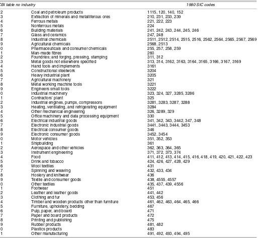
The vector of residuals from (6) is an estimate of the extent of second-hand markets for each three-digit industry. Using a correspondence table from the SIC to the CBI industry set (see App. A, Table A.1), we then derived measures for the set of CBI industries that comprise our sample. Because there is no strong case for interpreting the residual as a cardinal measure, we used its reverse ranking as an ordinal measure of irreversibil-ity (irrai). As a measure for comparison, we also computed the
reverse ranking of the ratio of the raw time-averaged figures (Di/Ai); we call this the unadjusted measure (irrbi). All
rank-ings are detailed in Appendix C. The rankrank-ings seem intuitively plausible. For example, the most irreversible industries include the process ones (chemicals and metals, building materials, rub-ber, plastic, paper and board, food, drink and tobacco), which all have high rankings; the reversible categories include light engineering, publishing, and most textile, clothing, leather, and wood industries, all of which have a relatively low rank.
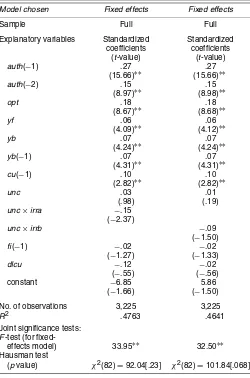
Next, we ran the machinery panel regression for the full set of industries, including both the uncertainty measure (unc) and the interaction ofuncwith the measure of irreversibility (irra
andirrb). The results, given in Table 3, show that extra lags onuncdo not contribute any explanatory power. There is clear
Driver, Temple, and Urga: Testing Real Options Theory 439
Table 3. Panel Estimation for Machinery
Model chosen Fixed effects Fixed effects
Sample Full Full No. of observations 3,225 3,225
R2 .4763 .4641 Joint significance tests:
F-test (for
fixed-effects model) 33.95∗∗ 32.50∗∗
Hausman test
(pvalue) χ2(82)=92.04[.23] χ2(82)=101.84[.068]
NOTE: See Table 2.
significance for the interaction effect withirra. It is signed neg-atively, in accordance with the prior expectation that greater ir-reversibility would strengthen the negative uncertainty effect. The interaction using the unadjusted ratio is significant at only the 10% level.
The results of these interactions may be compared with find-ings of Guiso and Parigi (1999), who using a different specifi-cation but with a set of irreversibility measures based on ease of disposal or availability of second-hand markets, obtained sim-ilar findings to ours. In particular, using a split sample based on access to second-hand markets, they found that “uncertainty is especially relevant whenever it is costly to dispose of excess capital” (p. 208).
7. CONCLUSIONS
In the light of real options theory, this article suggests that comparing investment across two classes of assets may provide important insights into the role of uncertainty. Specifically, we hypothesize that investment would be more in the nature of a sunk cost for machinery than for buildings, whereas buildings would be characterized by lower expandability due to higher expansion cost premia.
To test for real option effects, we report estimates of invest-ment authorization equations for both machinery and buildings,
focusing on contrasts among the (standardized) magnitude, sign, and significance of the uncertainty terms. We compared the results using SURE and panel estimation and found that the effect of uncertainty is different between machinery and build-ings. Several results stand out when both the asset panels are split into those industries with positive coefficients and those with negative coefficients. Specifically, the negative effect of uncertainty on machinery investment is much greater than for buildings for those industries with negative coefficients in the SURE estimation. At the same time, the positive effect of un-certainty is strongly significant for buildings and not significant for machinery for those industries with positive coefficients in the SURE estimation. These results support the theory of defer-ment options operating more strongly in the case of machinery and for expansion options operating more strongly in the case of buildings.
Additional results were presented for machinery, for which it proved possible to interact a specially constructed industry-specific proxy for irreversibility with the industry-industry-specific un-certainty term. This interaction was negative and significant, in line with the expectation of real options theory that irreversibil-ity should amplify the negative influence of uncertainty on fixed investment for this asset class.
To conclude, we restate the major overall finding of this study. This is that the contrast in investment between machinery assets and building assets is explainable as a contrast between the existence of deferment options and expansion options.
ACKNOWLEDGMENTS
The authors thank participants in seminars at the Australian National University, Canberra, the University of Melbourne, and the 10th International Conference on Panel Data in Berlin. They also thank the editor, Torben Andersen; the coeditor, Alis-tair Hall; an associate editor; and an anonymous referee for use-ful comments and suggestions that greatly improved the article. The usual disclaimer applies. K. Imai and J. Munoz Bugarin provided superb research assistance. Funding from the ESRC under grant R000223385 is gratefully acknowledged.
APPENDIX A: CBI DATA AND VARIABLE DEFINITIONS
A.1 The CBI Industrial Trends Survey
In this article we draw on the Industrial Trends Survey car-ried out by the main employers’ organization, the Confedera-tion of British Industry (CBI), with more than 1,000 replies on average each quarter. It has been published on a regular basis since 1958 and has been widely used by economists. Our panel dataset is restricted to the period 1978 Q1–1999 Q1, because the question on authorization of investment was added in 1978. The responses in the survey are weighted by net output, with the weights updated regularly. The survey sample is chosen to be representative and is not confined to CBI members:
√ Survey Questions
CBI Industrial Trends Survey Questions
√
Question 1
Are you more or less optimistic than you were 4 months ago about the general business situation in your industry?
√ Question 3b
Do you expect to authorize more or less capital expen-diture in the next 12 months than you authorized in the past 12 months on machinery? (possible choices: “more,” “same,” or “less”)
√ Question 4
Is your present level of output below capacity (i.e., are you working below a satisfactory full rate of operation)? (“yes” or “no”)
√
Question 8
Excluding seasonal variations, what has been the trend over the PAST 4 MONTHS, and what are the expected trends for the NEXT 4 MONTHS, with regard to volume of output? (“up,” “same,” or “down”)
√ Question 16c
Part C of this question invites respondents to consider which factors are “expected to limit capital expenditure
authorizations over the next 12 months.” We aggregate the following reply categories:
• A shortage of internal finance
• An inability to raise external finance.
A.2 Variable Definitions
The variables in (4) are constructed as transformations of the qualitative data in the survey using a balance of up (more) over down (less). (See Smith and McAleer 1995 and Driver and Urga 2004 for empirical validation of these transformations.)
auth: balance of more over less from Question 3b
ybandyf: balance of ups over downs (PAST and NEXT)
from Question 8, as explained below.
Table A.1. Industry Details
CBI table no industry 1980 SIC codes
22 Coal and petroleum products 1115, 120, 140, 152 23 Extraction of minerals and metalliferous ores 210, 231, 233, 239 24 Ferrous metals 221, 222, 223 25 Nonferrous metals 224
26 Building materials 241, 242, 243, 244, 245, 246 27 Glass and ceramics 247, 248
28 Industrial chemicals 2511, 2512, 2514, 2515, 2516, 2562, 2564, 2565, 2567, 2569 29 Agricultural chemicals 2568, 2513
30 Pharmaceuticals and consumer chemicals 255, 257, 258, 259 31 Man-made fibres 260
32 Foundries; and forging, pressing, stamping 311, 312
33 Metal goods not elsewhere specified 313, 314, 3162, 3163, 3164, 3165, 3166, 3167, 3169 34 Hand tools and implements 3161
35 Constructional steelwork 3204 36 Heavy industrial plant 3205 37 Agricultural machinery 321 38 Metal working machine tools 3221 39 Engineers small tools 3222
40 Industrial machinery 323, 324, 327, 3285, 3286 41 Contractors’ plant 325
42 Industrial engines, pumps, compressors 3281, 3283, 3287, 3288 43 Heating, ventilating, and refrigerating equipment 3284
44 Other mechanical engineering 326, 3289, 329 45 Office machinery and data processing equipment 330
46 Electrical industrial goods 341, 342, 343, 3442, 347, 348 47 Electronic industrial goods 3441, 3443, 3444, 3453 48 Electrical consumer goods 346
49 Electronic consumer goods 3452, 3454 50 Motor vehicles 351, 352, 353 51 Shipbuilding 361
52 Aerospace and other vehicles 362, 363, 364, 365 53 Instrument engineering 371, 372, 373, 374
54 Food 411, 412, 413, 414, 415, 416, 418, 419, 420, 421, 422, 423 55 Drink and tobacco 424, 426, 427, 428, 429
56 Wool textiles 431
57 Spinning and weaving 432, 433, 434 58 Hosiery and knitwear 436
59 Textile and consumer goods 438, 4555, 4557 60 Other textiles 435, 437, 439, 4556
61 Footwear 451
62 Leather and leather goods 441, 442 63 Clothing and fur 453, 456
64 Timber and wooden products other than furniture 461, 462, 463, 464, 465, 466 65 Furniture, upholstery, bedding 467
66 Pulp, paper, and board 471 67 Paper and board products 472 68 Printing and publishing 475 69 Rubber products 481, 482 70 Plastics products 483
71 Other manufacturing 491, 492, 493, 494, 495
Driver, Temple, and Urga: Testing Real Options Theory 441
Specifically, the first term on the right side of (2) is obtained using a Taylor approximation as
logYt=
logYt−
Yt−1 Yt
=
logYt+
Yt−Yt−1
Yt −
1
≈[logYt+logYt]
= [logYt+logYt]. (A.1)
This is equal to the sum of the survey balance plus the first dif-ference of that balance. Thus this is the termytin (3), two
ver-sions of which (yb, backward, andyf, forward) are used in (4).
opt: balance of more over less from Question 1
fi: responses to internal and external finance constraints from Question 16c
cu: based on logit of % “no” response from Question 4, as discussed below.
The equilibrium correction term in (2) and (3) is obtained by proxying the unknownlevelof authorizationsAtby the change
in the capital stock(Kt), on the assumption of proportional
depreciation and in the light of the close correspondence be-tween authorized and actual investment found from the realiza-tion studies cited in the text. Writing
log(K/Y)t−1=log[(Kt−1/Yt−1)−(Kt−2/Yt−1)].
Using a Taylor approximation, we may write the right side term as
[log(Kt−1/Yt−1)] −(Kt−2/Kt−1)
= [logKt−1−logYt−1] +(Kt−1−Kt−2)/Kt−1−1 ≈logKt−1−logYt−1+logKt−1−1.
Again, using a Taylor approximation for logYt−1
(=logYt−1−Yt−2/Yt−1),
=logKt−1−logYt−1+Yt−2/Yt−1+logKt−1−1 ≈log(K/Y)t−1+log(K/Y)t−1
= −[log(Y/K)+log(Y/K)]t−1, (A.2)
where(Y/K)t is an indicator of capacity utilization measured
from the survey as the logit of the percentage of firms reporting capacity utilization above normal (% answering “no” to Ques-tion 4 of the survey). The expression in (A.2) is thus calculated as the logit of Question 4 (“no”) plus the first difference of this logit. This combined term is the termcut−1in (3).
dlcu: first difference term in logit of % “no” response from Question 4
unc: based on responses to the survey question on in-dustry optimism, Question 1. Specifically, this is the entropy of the three replies (up/same/down). WritingSjfor the share of replyj,j=1,3, we
de-fine unc=
[−SjlogSj]. An even spread in the
replies (each share Si equal to one-third)
corre-sponds to maximum entropy and maximum uncer-tainty. It may be noted that the question relates to optimism with respect to the industry rather than the firm, so that the dispersion recorded should not reflect different objective circumstances, but rather different expectations in respect of a com-mon variable.
[Received October 2003. Revised November 2005.]
APPENDIX B: SUMMARY STATISTICS ON UNRESTRICTED SURE RESULTS
Machinery Buildings
CBI classification and industry R2 DW R2 DW
24 Ferrous metals .63 1.85 .56 1.90 25 Nonferrous metals .49 1.79 .34 2.15 26 Building materials .71 2.15 .56 1.80 27 Glass and ceramics .81 2.25 .77 2.05 28 Industrial chemicals .57 2.04 .46 2.04 30 Pharmaceuticals and consumer chemicals .42 2.11 .41 1.86 32 Foundries; and forging, pressing, and stamping .67 2.11 .68 2.00 33 Metals goods n.e.s. .77 2.28 .65 1.87 34 Hand tools and implements .69 2.20 .61 2.19 35 Constructional steelwork .66 2.13 .44 1.88 36 Heavy industrial plant .19 2.08 .14 2.09 37 Agricultural machinery .51 1.80 .28 1.92 38 Metal working machine tools .54 2.23 .47 2.13 39 Engineer’s small tools .63 1.79 .62 2.11 40 Industrial machinery .50 2.46 .54 2.20 41 Contractors’ plant .63 1.58 .61 1.99 42 Industrial engines, pumps, and compressors .52 1.69 .39 2.04 43 Heating, ventilating, and refrigerating equipment .53 2.17 .51 1.73 44 Other mechanical equipment .73 2.13 .47 1.99 46 Electrical industrial goods .39 2.02 .24 2.29* 47 Electronic industrial goods .41 2.21 .29 1.99 48 Electrical consumer goods .58 1.90 .34 2.11 49 Electronic consumer goods .35 1.99 .28 1.79 50 Motor vehicles .58 2.28 .40 2.02 52 Aerospace and other vehicles .38 1.89 .42 2.06 53 Instrument engineering .41 1.83 .31 2.24
54 Food .34 2.25 .49 2.25
55 Drink and tobacco .26 1.86 .26 1.89 56 Wool textiles .58 2.19 .59 2.01
APPENDIX B (continued)
Machinery Buildings
CBI classification and industry R2 DW R2 DW
57 Spinning and weaving .69 1.64 .38 1.84 58 Hosiery and knitwear .51 1.69 .28 2.04 59 Textile consumer goods .38 2.21 .48 1.98
61 Footwear .54 2.27 .48 2.33
62 Leather and leather goods .67 2.04 .67 2.05 63 Closing and fur .63 2.02 .61 1.90 64 Timber and wooden products other than furniture .69 1.99 .70 1.94 65 Furniture, upholstery, and bedding .68 2.25 .65 2.39 66 Pulp, paper, and board .52 1.95 .38 1.92 67 Paper and board products .51 2.05 .50 2.10 68 Printing and publishing .56 2.35 .40 1.92 69 Rubber products .58 2.00 .57 2.23 70 Plastic products .61 2.06 .51 2.15
APPENDIX C: COMPOSITION OF PANELS AND RANKING OF D
/
A (DISPOSAL AND ACQUISITION RATIO) AT INDUSTRY LEVELIndustries Industries Industries Industries Reverse Reverse with negative with positive with negative with positive ranking of adjusted and significant and significant and significant and significant D/A ranking of coefficient in coefficient in coefficient in coefficient in (irra)∗ D/A
SURE estimation SURE estimation SURE estimation SURE estimation (irrb) Estimation for Estimation for Estimation for Estimation for
machinery machinery building building CBI classification and industry∗ investment investment investment investment
23 Coal and petroleum product 30 19
24 Ferrous metals 43 44
25 Nonferrous metals 40 34
26 Building materials X 38 37
27 Glass and ceramics 41 38
28 Industrial chemicals X 24 45 30 Pharmaceuticals and consumer chemicals X X 39 41 32 Foundries; and forging, pressing, and stamping 31 24 33 Metals goods n.e.s. X 14 23 35 Constructional steelwork X X 12 9 36 Heavy industrial plant X 13 10 37 Agricultural machinery 42 36 38 Metal working machine tools 2 2 39 Engineer’s small tools X 3 3
40 Industrial machinery 9 20
41 Contractors’ plant 6 4
42 Industrial engines, pumps, and compressors X X 19 27 43 Heating, ventilating, and refregiating equipment X 20 28 44 Other mechanical equipment X 11 25 45 Office machinery and data processing 21 16 46 Electrical industrial goods 10 31 47 Electronic industrial goods X X 23 30 48 Electrical consumer goods 44
49 Electronic consumer goods X X 22 22
50 Motor vehicles 18 43
51 Shipbuilding 15 11
52 Aerospace and other vehicles 36 33 53 Instrument engineering 27 21
54 Food X X 26 39
55 Drink and tobacco X X 34 35
56 Wool textiles 8 7
57 Spinning and weaving X 7 5 58 Hosiery and knitwear X 1 1 59 Textile consumer goods 37 29
61 Footwear 33 17
62 Leather and leather goods 32 14
63 Closing and fur 17 12
64 Timber and wooden products other than furniture X X 16 13 65 Furniture, upholstery, and bedding 25 15 66 Pulp, paper, and board X X 45 42 67 Paper and board products X 5 6 68 Printing and publishing 4 8 69 Rubber products X X
70 Plastic products 28 32
∗Industries that are omitted from the table are those with missing observations for either CBI survey data for the data on disposal or acquisition.
Driver, Temple, and Urga: Testing Real Options Theory 443
REFERENCES
Abel, A. B., Dixit, A. K., Eberly, J. C., and Pindyck, R. S. (1996), “Options, the Value of Capital and Investment,”Quarterly Journal of Economics, 111, 753–777.
Asplund, M. (2000), “What Fraction of a Capital Investment Is Sunk Cost?”
Journal of Industrial Economics, 48, 287–304.
Bar-Ilan, A., and Strange, W. C. (1996), “Investment Lags,”American Eco-nomic Review, 86, 610–622.
Bera, A. K., and McAleer, M. (1989), “Nested and Non-Nested Procedures for Testing Linear and Log-Linear Regression Models,”Sankhy¯a, Ser. B, 51, 212–224.
Bernanke, B. S. (1983), “Irreversibility, Uncertainty and Cyclical Investment,”
Quarterly Journal of Economics, 98, 85–106.
Berndt, E. R. (1990),The Practice of Econometrics: Classic and Contempo-rary, Reading, MA: Addison-Wesley.
Breusch, T. S., and Pagan, A. R. (1980), “The Lagrange Multiplier Test and Its Applications to Model Specification in Econometrics,”Review of Economic Studies, 47, 239–254.
Caballero, R. (1999), “Aggregate Investment,” inHandbook of Macroeco-nomics, Vol. 1, eds. J. B. Taylor and M. Woodford, Amsterdam: North Hol-land, pp. 813–862.
Chatelain, J. B., and Teurlai, J. C. (2001), “Pitfalls in Investment Euler Equa-tions,”Economic Modelling, 18, 159–179.
Chirinko, R. S. (1993), “Business Fixed Investment Spending: Modelling Strategies, Empirical Results and Policy Implications,”Journal of Economic Literature, 31, 1875–1911.
Chirinko, R. S., Fazzari, S. M., and Meyer, A. P. (1999), “How Responsive Is Business Capital Formation to Its User Cost? An Explanation With Micro Data,”Journal of Public Economics, 74, 53–80.
Dixit, A., and Pindyck, R. (1994),Investment Under Uncertainty, Princeton, NJ: Princeton University Press.
Driver, C., and Meade, N. (2001), “Persistence of Capacity Shortage and the Role of Adjustment Costs,”Scottish Journal of Political Economy, 48, 27–47.
Driver, C., and Urga, G. (2004), “Transforming Qualitative Survey Data: Per-formance Comparison for the U.K.,”Oxford Bulletin of Economics and Sta-tistics, 66, 71–89.
European Commission (1997), “The Joint-Harmonised EU Programme of Busi-ness and Consumer Surveys,”European Economy, 6, Brussels.
Fuchs, V. R., Krueger, A. B., and Poterba, J. M. (1998), “Economists’ Views About Parameters, Values, and Policies: Survey Results in Labor and Public Economics,”Journal of Economic Literature, 36, 1387–1425.
Garber, P., and King, R. (1983), “Deep Structural Excavation? A Critique of Euler Equation Methods,” Working Paper 31, National Bureau of Economic Research.
Ghosal, V. (2002), “The Impact of Uncertainty and Sunk Costs on Firm Dynam-ics and Industry Structure: Evidence From the U.S. Manufacturing Sector,” CIC Working Paper SPII2003-12, Wissenschaftszentrum Berlin.
Giordani, P., and Soderland, P. (2003), “Inflation Forecast Uncertainty,” Euro-pean Economic Review, 47, 1037–1059.
Government Statistical Service (1986), “Commercial and Industrial Floorspace Statistics: England 1982-5,” Department of the Environment Report 14, HMSO.
Guiso, L., and Parigi, G. (1999), “Investment and Demand Uncertainty,”The Quarterly Journal of Economics, 115, 185–227.
Hulten, C. R., and Wykoff, F. C. (1981), “The Estimation of Economic Depre-ciation Using Vintage Asset Prices: An Application of the Box–Cox Power Transformation,”Journal of Econometrics, 15, 367–396.
Judge, G. G., Hill, R. C., Griffiths, W. E., Lutkepohl, H., and Lee, T. C. (1988),
Introduction to Theory and Practice of Econometrics(2nd ed.), New York: Wiley.
Kessides, I. N. (1990a), “Market Concentration, Contestability, and Sunk Costs,”Review of Economics and Statistics, 72, 614–622.
(1990b), “Towards a Testable Model of Entry: A Study of U.S. Manu-facturing Industries,”Economica, 57, 219–238.
Lamont, O. A. (2000), “Investment Plans and Stock Returns,”Journal of Fi-nance, 55, 2719–2745.
Lensink, R., Bo, H., and Sterken, E. (2001),Investment, Capital Market Imper-fections and Uncertainty, London: Edward Elgar.
MacKinnon, J. G., White, H., and Davidson, R. (1983), “Tests for Model Spec-ification in the Presence of Alternative Hypothesis: Some Further Results,”
Journal of Econometrics, 21, 53–70.
Mairesse, J., Hall, B. H., and Mulkay, B. (1999), “Firm-Level Investment in France and the United States: An Exploration of What We Have Learned in Twenty Years,” Working Paper 7437, National Bureau of Economic Re-search.
Ramey, V. A., and Shapiro, M. D. (2001), “Displaced Capital: A Study of Aerospace Plant Closings,”Journal of Political Economy, 109, 958–992. Smith, J., and McAleer, M. (1995), “Alternative Procedures for
Convert-ing Qualitative Response Data to Quantitative Expectations: An Applica-tion to Australian Manufacturing,”Journal of Applied Econometrics, 10, 165–185.
Sutton, J. (1991), Sunk Cost and Market Structure, Cambridge, MA: MIT Press.
Worthington, P. R. (1995), “Investment, Cash Flow and Sunk Costs,”Journal of Industrial Economics, 153, 49–61.
Zarnowitz, V., and Lambros, L. A. (1987), “Consensus and Uncer-tainty in Economic Prediction,” Journal of Political Economy, 95, 591–621.