Full Terms & Conditions of access and use can be found at
http://www.tandfonline.com/action/journalInformation?journalCode=ubes20
Download by: [Universitas Maritim Raja Ali Haji] Date: 12 January 2016, At: 23:32
Journal of Business & Economic Statistics
ISSN: 0735-0015 (Print) 1537-2707 (Online) Journal homepage: http://www.tandfonline.com/loi/ubes20
Tracking the Business Cycle of the Euro Area
João Valle e Azevedo, Siem Jan Koopman & António Rua
To cite this article: João Valle e Azevedo, Siem Jan Koopman & António Rua (2006) Tracking the Business Cycle of the Euro Area, Journal of Business & Economic Statistics, 24:3, 278-290, DOI: 10.1198/073500105000000261
To link to this article: http://dx.doi.org/10.1198/073500105000000261
Published online: 01 Jan 2012.
Submit your article to this journal
Article views: 115
Tracking the Business Cycle of the Euro Area:
A Multivariate Model-Based Bandpass Filter
João V
ALLE EA
ZEVEDODepartment of Economics, Stanford University, Stanford, CA 94305-6072 (azevedoj@stanford.edu)
Siem Jan K
OOPMANDepartment of Econometrics, Vrije Universiteit Amsterdam, 1081 HV Amsterdam, The Netherlands (s.j.koopman@feweb.vu.nl)
António R
UAEconomic Research Department, Banco de Portugal, 1150-012 Lisboa, Portugal (antonio.rua@bportugal.pt)
This article proposes a multivariate bandpass filter based on the trend plus cycle decomposition model. The underlying multivariate dynamic factor model relies on specific formulations for trend and cycle com-ponents and produces smooth business cycle indicators with bandpass filter properties. Furthermore, cycle shifts for individual time series are incorporated as part of the multivariate model and estimated simulta-neously with the remaining parameters. The inclusion of leading, coincident, and lagging variables for the measurement of the business cycle is therefore possible without a prior analysis of lead–lag relationships between economic variables. This method also permits the inclusion of time series recorded with mixed frequencies. For example, quarterly and monthly time series can be considered simultaneously without ad hoc interpolations. The multivariate approach leads to a business cycle indicator that is less subject to revisions than those produced by univariate filters. The reduction of revisions is a key feature in real-time assessment of the economy. Finally, the proposed method computes a growth indicator as a byproduct. The new approach of tracking business cycle and growth indicators is illustrated in detail for the Euro area. The analysis is based on nine key economic time series.
KEY WORDS: Bandpass filter; Business cycle; Dynamic factor model; Kalman filter; Phase shift; Re-visions; Unobserved components time series model.
1. INTRODUCTION
Designing fiscal and monetary policies requires information about the state of the economy. Given the importance of this knowledge for the policy maker, a clear economic picture is needed at all times. However, the assessment of the economic situation can be a challenging task when one faces noisy data giving mixed signals about the overall state of the economy. To avoid a solely judgment-based procedure in the economic analysis, one should be able to extract the relevant informa-tion through a statistical rigorous method capable of providing a clear signal regarding current economic developments.
A business cycle indicator aims to present deviations from a long-term trend in economic activity. Such deviations typically last between 1.5 and 8 years. The time series of real gross do-mestic product (GDP) is undoubtedly one of the most important variables in business cycle assessment. For example, Stock and Watson (1999) stated that “fluctuations in aggregate output are at the core of the business cycle, so the cyclical component of real GDP is a useful proxy for the overall business cycle.” Com-mon practice is to signal extract the cycle from real GDP us-ing a nonparametric filter, such as that of Hodrick and Prescott (1997) or of Baxter and King (1999). These filters are based on symmetric weighting kernels and provide consistent methods of extracting trends and cycles in the middle of the time series but encounter problems at the beginning and end of the series. The Baxter and King (1999) filter is called a bandpass filter, because it aims to extract the dynamics that are strictly associated with the business cycle frequencies 2π/p, with pranging from 1.5 to 8 years. The optimality of bandpass filters is evaluated in the frequency domain by investigating gain functions that should
affect only the business cycle frequencies. Recently, Christiano and Fitzgerald (2003) developed an almost optimal filter in this respect, together with a solution to the endpoints problem.
The signal extraction of a business cycle can also be based on formulating an unobserved components time series models for real GDP, as was done by Clark (1987) and Harvey and Jaeger (1993). Recently, Harvey and Trimbur (2003) presented a new class of model-based filters for extracting trends and cycles in economic time series. The main feature of these model-based filters is that it is possible to extract a smooth cycle from eco-nomic time series. It is shown that the implied filters from this class of models have bandpass filter properties similar to those of the filter of Baxter and King (1999). Furthermore, model-based filters provide a mutually consistent way to extract trends and cycles even at the beginning and end of the series. But the univariate approaches of bandpass and model-based filters do not exploit the information stemming from several economic time series. Recently, Forni, Hallin, Lippi, and Reichlin (2000) and Stock and Watson (2002) showed that business cycle and growth indicators can be obtained from hundreds of economic time series. Such an approach is in sharp contrast with the com-mon practice of using univariate bandpass filters and univariate model-based methods for obtaining business cycle indicators. In this article we aim to take a position between the “all or one” strategy by considering a moderate set of time series instead of considering real GDP only or considering a vast amount of
© 2006 American Statistical Association Journal of Business & Economic Statistics July 2006, Vol. 24, No. 3 DOI 10.1198/073500105000000261 278
time series. Our approach requires maintaining of a moderate database of, say, nine time series.
When considering trends and cycles in multivariate time se-ries, we also need to focus on possible lead–lag relationships between variables and the business cycle. We therefore incor-porate the phase-shift mechanism of Rünstler (2004) for in-dividual cycles with respect to the base cycle modeled as the generalized cycle component of Harvey and Trimbur (2003). This development enables the simultaneous modeling of lead-ing, coincident, and lagging indicators for the business cycle without their a priori classification. As a result, phase shifts are estimated as parameters of the model. This contrasts with the multivariate model-based analysis of Stock and Watson (1989), where the coincident indicator is defined as the common factor of a small set of coincident variables identified before estima-tion. The treatment of phase shifts in a model-based approach allows the exploitation of information contained in both lags and leads of variables for computing the business cycle indi-cator, and it overcomes the restriction of using only coincident variables.
Economic and financial policy decision makers need a busi-ness cycle indicator at a high frequency despite the fact that time series information is usually not available at the desired frequency. But information recorded at a lower frequency must not be discarded. The crucial example refers to the time se-ries of real GDP that was disregarded by Stock and Watson (1989) when constructing its composite indicator, presumably because it is available only on a quarterly basis. Others, includ-ing Altissimo, Bassanetti, Cristadoro, Forni, Lippi, Reichlin, and Veronese (2001), handled this shortcoming by considering a monthly interpolated GDP series. In the multivariate analy-sis of this article, observations of different frequencies can be incorporated because missing observations can be treated by the implemented state-space methods. The ability to deal with missing observations also ensures that the business cycle indi-cator will be up-to-date even when long delays in data releases are present. This feature is important given the significant data release delays in the Euro area.
In this article we develop a feasible procedure for the com-putation of business cycle indicators. The resulting business cy-cle filter is based on a multivariate dynamic factor model for a vector of economic and monetary time series recorded at quar-terly and monthly frequencies. The dynamic specification of the model allows the latent factors to be interpreted as trend and cycle components. The common cycle component is formu-lated as done by Harvey and Trimbur (2003) and can be shifted for individual variables as done by Rünstler (2004). The sig-nal extraction of the cycle component can be considered the re-sult of a multivariate model-based approximate bandpass filter. The multivariate procedure is shown to produce a cycle indi-cator that is subject to smaller revisions compared to univari-ate bandpass filters and univariunivari-ate model-based filters. Hence the real-time signal extraction has been improved against com-monly used filters in business cycle analysis. This key feature is important for macroeconomic stabilization policy decisions, because reliable estimates of the business cycle position in real time are crucial in this respect.
We implement the multivariate model-based bandpass filter for business cycle tracking of the Euro area. By pooling in-formation from nine key economic variables (including GDP,
industrial production, retail sales, confidence indicators, and others) it obtains a business cycle indicator in line with com-mon wisdom regarding Euro area business cycle developments. The business cycle indicator can be considered a monthly proxy for the output gap. A growth indicator can also be constructed from our analysis as a byproduct and is compared with the EuroCOIN indicator. This growth indicator of Altissimo et al. (2001) is based on a generalized dynamic factor model with almost 1,000 economic series as input. The parsimonious ap-proach proposed in this article leads to a similar growth indica-tor and overcomes some drawbacks of EuroCOIN.
The article is organized as follows. In Section 2 we present the underlying dynamic factor model and its extensions. In Sec-tion 3 we proceed to the empirical applicaSec-tion for the Euro area. We conclude in Section 4.
2. MODEL FOR MULTIVARIATE BANDPASS FILTERING
Assume that a panel ofNeconomic time series is collected in theN×1 vectorytand that we observendata points over time,
that is,t=1, . . . ,n. Theith element of the observation vector at timetis denoted byyit.
2.1 The Basic Trend-Cycle Decomposition Model
The basic unobserved components time series model for measuring the business cycle from a panel of economic time series is based on the decomposition model
yit=µit+δiψt+εit, i=1, . . . ,N,t=1, . . . ,n, (1)
whereµitis the individual trend component for theith time
se-ries andψt denotes the business cycle component (common to
all time series). For each series, the contribution of the cycle is measured by the coefficient δi for i=1, . . . ,N. The
idio-syncratic disturbance εit is assumed normal and independent
from εjs for i=j and/or t=s. The variance of the irregular
disturbance varies for the different individual series, that is,
εit
iid
∼N(0, σi2,ε), i=1, . . . ,N. (2) Each trend component from the panel time series is specified as the local linear trend component (see Harvey 1989), that is,
µi,t+1=µit+βit+ηit, ηit
mutually independent of each other and other disturbances, at all time points and across theNequations. Therefore the trends are independent of each other within the panel. The cycle com-ponent is common to all time series in the panel and can be specified as an autoregressive model with polynomial coeffi-cients that have complex roots. Specifically, we enforce this restriction by formulating the cycle time series process as a trigonometric process, that is,
whereκtandκt+are white noise disturbances and mutually
in-dependent of each other at all time points fort=1, . . . ,n. The damping term 0< φ≤1 ensures that the stochastic processψt
is stationary or fixed as the cycle variance is specified asσκ2=
(1−φ2)σψ2, whereσψ2 is the variance of the cycle. The period of the stochastic cycle is defined as 2π/λ, where 0≤λ≤π is approximately the frequency at which the spectrum of the sto-chastic cycle has the largest mass. The initial distribution of the cycle is given by can be characterized through the autocovariance function given by
γ (τ )=E(ψtψt−τ)=σκ2φ τ
(1−φ2)−1cos(λτ ), forτ =0,1,2, . . ..
2.2 Signal Extraction and Weights Bandpass Filter Properties
The basic trend-cycle decomposition model falls within the class of multivariate unobserved components time series models or multivariate structural time series models that can be cast in state-space form. The details of this general class of multivariate models have been discussed by Harvey and Koopman (1997), including its relations with other multivari-ate approaches, such as the common feature models of Engle and Kozicki (1993). Furthermore, Harvey and Koopman (2000) discussed vector autoregressive model representations of un-observed component models that are related to the canonical correlation analyses of Tiao and Tsay (1985) and the multiple time series analyses of Ahn and Reinsel (1988). The unknown parameters, such as variances associated with the disturbances of the model and loading factor coefficientsδifor the common
cycle component, are estimated by numerically maximizing the likelihood function evaluated by the Kalman filter. The signal extraction of unobserved trend and cycle components is carried out by the Kalman filter and associated smoothing methods. An introduction to such techniques was given by, for example, Harvey (1989) and Durbin and Koopman (2001).
It may be of interest to know how observations are weighted when, for example, the business cycle estimate at timetis con-structed. Such weights can be obtained as discussed by Harvey and Koopman (2000). The implications of the filter in the fre-quency domain can be assessed through the spectral gain func-tion (see Harvey 1993, chap. 6). A filter is said to havebandpass filter propertieswhen the gain function has sharp cutoffs at both ends of the range of business cycle frequencies.
2.3 Generalized Components
The basic trend plus cycle decomposition model (1) can be modified in such a way that the model-based filtering and smoothing method has bandpass filter properties (see Gomez 2001; Harvey and Trimbur 2003). For example, themth-order stochastic trend for series i can be considered as given by µit=µ(itm), where trend specification (6) can be taken as the model representa-tion of the class of Butterworth filters commonly used in engi-neering (see Gomez 2001). The special case of (6) withm=2 reduces to the local linear trend component (3) withσi2,η=0, from which it follows thatβit =µ(it1). The effect of a higher
value formis pronounced in the frequency domain because the low-pass gain function will have a sharper cutoff downward at a certain low frequency point. In the time domain the effect is evident, becausemµ(i,mt+)1=ζitsuggests that the time seriesyit
implied by model (1) and (6) must be differencedmtimes to become stationary. From this perspective, the choice of a rel-atively large choice formthus may not be realistic for many economic time series.
The generalized specification for thekth-order common cy-cle component is given byψt=ψt(k), where cutoffs of the bandpass gain function at both ends of the range of business cycle frequencies centered atλ. For example, the model-based filter withk=6 leads to a similar gain function as that of Baxter and King (1999) (see Harvey and Trimbur 2003). However, by increasingk, there is a trade-off between the sharp-ness of the implicit bandpass filter and its behavior at the end-points of the sample. A sharper cutoff implies larger revisions of the estimates near the endpoints, because more weight is given to the (implicitly forecasted) observations in the far future. In the empirical study of this article, a good compromise is found atk=6, although smaller values ofkdid not lead to completely different estimates of the key parameters in the model. Differ-ent variations within this class of generalized cycles have been discussed by Harvey and Trimbur (2003), who referred to spec-ification (8) as the balanced cycle model. They preferred this specification because deriving the time-domain properties of cycleψt is more straightforward and the specification tends to
give a slightly better fit to a selection of U.S. economic time se-ries. The number of unknown parameters remains three for cy-cle specification (4), that is, 0< φ≤1, 0≤λ≤π, andσκ2>0, for any orderk.
2.4 Phase Shifts of the Business Cycle
In the multivariate case, withN>1, multiple time series are considered for the construction of a business cycle indicator. The contribution of theith time series to cycleψtis determined
by loadingδi, for i=1, . . . ,N. In the current model (1) with
generalized trend and cycle components, only economic time series with coincident cycles are viable candidates for inclusion
into the model. Prior analysis may determine whether includ-ing leads or lags of economic variables is appropriate. To avoid such a prior analysis, the model is modified to allow the base cycleψtto be shifted for each time series. For this purpose, we
adopt the phase-shift mechanism for a multivariate cycle speci-fication as proposed by Rünstler (2004). For a given cycle com-ponent given by (4), it follows from a standard trigonometric identity that the autocovariance function of cycleψt is shifted
ξ0time periods to the right (whenξ0>0) or to the left (when ξ0<0) by considering
cos(ξ0λ)ψt+sin(ξ0λ)ψt+, t=1, . . . ,n.
The shiftξ0is measured in real time, so thatξ0λis measured in radians, and due to the periodicity of trigonometric functions, the parameter space ofξ0is restricted within the range−12π < ξ0λ <12π. For example, it follows that when a cosine is shifted by xλ, its correlation with the base cosine is the same as its correlation with a cosine that is shifted by(π−x)λ, but with an opposite sign, for12π <xλ < π. The shifted cycle is introduced in the decomposition model by replacing (1) with
yit=µ(itm)+δicos(ξiλ)ψt(k)+sin(ξiλ)ψt+(k)
+εit,
i=1, . . . ,N,t=1, . . . ,n, (9) where the specifications in (6), (8), and (2) remain applicable. Rünstler (2004) showed that the phase shift appears directly as a shift in the autocovariance function of the stochastic cycle. This remains to hold for model specification (9); see Appendix A for more details. We further restrict attention to a common cycle specification. It is assumed that the first equation identifies the base cycle and thusξ1=0 andδ1=1, so that
y1t=µ1t+ψt+ε1t, t=1, . . . ,n.
The common cycleψt coincides contemporaneously with the
first variable in the vectoryt. The restrictionδ1=1 can be re-placed by the constraint of a fixed value forσκ2. The restriction ξ1=0 allows the cycles of other variables to shift with respect to the cycle of the first variable. The general multivariate trend-cycle decomposition model can be formulated in state space with partially diffuse initial conditions. The details are given in Appendix B.
2.5 Some Further Issues
The multivariate trend-cycle decomposition model contains a common cycle specified as a generalized cycle and is allowed to shift for every individual series with respect to a base cycle. The generalized cycle specification is taken from Harvey and Trimbur (2003), and the phase-shift mechanism is taken from Rünstler (2004). The trend and irregular components in the model are idiosyncratic factors that account for the dynamics in the noncyclical range of frequencies in the time series. The model is cast in the state-space framework; therefore, variables with different observation frequencies in the panel can be han-dled straightforwardly using the Kalman filter (see Durbin and Koopman 2001, sec. 4.6). For example, the treatment of quar-terly time series using a monthly time index in the state-space framework amounts to having two consecutive monthly obser-vations as missing followed by the quarterly observation. There are alternative ways to account for mixed frequencies (see, e.g.,
Mariano and Murasawa 2003). Such solutions require nonlin-ear techniques, because macroeconomic time series are often modeled in logs. Our main interest is to capture the cycle and growth dynamics. Therefore, the different solutions will have a minor impact on the extracted cycle.
The specification of the dynamic factor model (9) can be ex-tended to a more general setting. Nevertheless, the key features of business cycle analysis are incorporated in the model. The generalized cycle enables us to interpret the extracted cycle as the result of an approximate bandpass filter to the reference se-ries in the spirit of Harvey and Trimbur (2003). As a result, the model can be viewed partly as a filtering device and partly as a specification of the true data-generating process. When we take the cycle of a particular series as the base cycle and we enforce the base cycle on the other series (adjusted for scale and phase) as in the proposed model specification, we effectively use infor-mation from the cyclical fluctuations of the other series only to the extent to which they match those of the series originally at-tached to the base cycle. Subject to phase-shift adjustments, the cyclical components of the various series are perfectly corre-lated. The bandpass filter interpretation is therefore warranted. We should note that cross-correlations (adjusted for phase) can be equal to unity only if the phase shift implies an integer shift in the cross-correlation function; see Appendix A. An integer shift is unlikely to occur in practice, because the shift parame-ter is a typical noninteger value and must be estimated. These insights into the model indicate that the model is appropriate for the purpose of the analysis: to obtain a business cycle indicator that is close to the one obtained from a univariate bandpass fil-ter but has betfil-ter properties in fil-terms of revision and availability at a higher frequency.
The identification of the parameters in the model is guaran-teed, because they all appear in the autocovariance function of the model in its reduced form. These results are standard for the multivariate unobserved components time series model, of which our model without cycle phase shifts is a special case (see Harvey and Koopman 1997). The identification of para-meters associated with cycle shifts was discussed by Rünstler (2004, prop. 2) and requires a unique decomposition for the autocovariance function of the cycle component. The specifica-tion that we have adopted is a special and simplified case of the Choleski decomposition.
3. EMPIRICAL RESULTS FOR THE EURO AREA
3.1 Data
The multivariate framework presented in the previous section allows the simultaneous modeling of leading, coincident, and lagging indicators for the business cycle with phase shifts esti-mated as an integrated part of the modeling process. However, as a preliminary step, one must define the base cycle. We follow Stock and Watson (1999), who considered the cyclical compo-nent of real GDP as a useful proxy for the overall business cy-cle. Therefore, we impose a unit common cycle loading and a zero phase shift for Euro area real GDP. The remaining series included in the multivariate analysis are the most commonly used monthly indicators on Euro area economic monitoring, in-cluding industrial production, retail sales, unemployment, sev-eral confidence indicators (consumers, industrial, retail trade,
Figure 1. Nine Key Economic Variables for the Euro Area, 1986–2002 [ GDP; IPI; interest rate spread; construction
con-fidence indicator; consumer confidence indicator; retail sales; unemployment (inverted sign); industrial confidence indicator;
retail trade confidence indicator].
and construction), and interest rate spread. As is well known, industrial production is highly correlated with the business cy-cle and is coincident or even slightly leading. In contrast, re-tail sales provide information about private consumption, which accounts for a large proportion of GDP. Unemployment is a countercyclical and lagging variable, but it also has a high cor-relation with the business cycle. Confidence indicators provide information regarding economic agents’ assessment of current and future economic situation, so they are expected to present coincident or leading properties. Finally, the interest rate spread has been widely recognized as a forward-looking indicator for real activity. These time series are available for the period 1986–2002 and are graphically presented in Figure 1. The re-sulting dataset covers different economic sectors and it is based on both quantitative and qualitative data, as well as on both real and monetary variables. GDP is available on a quarterly basis, whereas the other indicators are monthly. Appendix C provides a detailed description of the data.
3.2 Details of the Model for Multivariate Bandpass Filtering
The empirical study of the Euro area business cycle is based on the multivariate model (9) with generalized trendµit, given
by specification (6) withm=2, and common cycle ψt, given
by specification (8) withk=6. The first time series in the panel is real GDP. The time index refers to months and applies to all series in the panel except for GDP, which is observed every quarter. This implies that the monthly series of GDP has two consecutive monthly observations as missing followed by its quarterly observation.
A preliminary analysis of the panel of time series using band-pass filters reveals that cyclical correlations of the various series
with GDP ranges from.70 to.95. This range of correlation val-ues is relatively high, and we do not expect the model to capture this perfectly. But it does justify, to some extent, the decompo-sition model with a common base cycle and with trend and ir-regular components that account for the other dynamics in the series.
Harvey and Trimbur (2003) showed that the choice ofm=2 andk=6 leads to estimated trend and cycle components with bandpass filtering properties similar to the ones of Baxter and King (1999). The role of the trend componentµit in model (9)
is to capture the persistence of the time series excluding the cycle. The ordermof the trend (6) applies to all time series in the panel.
The frequency of the common cycle component is fixed to ensure that the cycle captures the typical business cycle pe-riod in the time series. Therefore, the frequency is chosen as λ=.06545, which implies a period of 96 months (8 years) and is consistent with the values reported by Stock and Watson (1999) for the U.S. and the European Central Bank (2001) for the Euro area. The frequency parameter is fixed to guarantee the extraction of typical business cycle fluctuations. When ap-plying bandpass filters to a typical integrated series, the peak in the spectrum of the filtered series is reached at the lowest fre-quency of the band of interest. Thus the value ofλis chosen to correspond approximately with the location of the peak in the spectrum. The choice is not based on minimizing the difference of the gain function between an ideal filter and a filter that is implicitly given by the model.
Further, we note thatδ1andξ1, the load and shift parameters associated with the base series, GDP, are restricted to 1 and 0. Apart from these restrictions, the number of parameters to es-timate for each equation is four (σi2,ζ,δi,ξi, andσi2,ε) and that
for the common cycle is two (φandσκ2). Thus the total number is 4N (4 for each equation minus 2 restrictions plus 2 for the common cycle).
The maximum likelihood estimates of the parameters are obtained by maximizing the log-likelihood function that is eval-uated through the Kalman filter. This is a standard exercise although computational complexities may arise because the parameter dimension rises quickly asN increases. For exam-ple, with N=9, the number of parameters to be estimated is 36. In principle, there is no difficulty of being able to em-pirically identify the parameters from the data because the number of observations increases accordingly with N. How-ever, it can be computationally and numerically cumbersome to obtain the maximum value of the log-likelihood function in a 36-dimensional space. A practical and feasible approach to overcome some numerical difficulties is to obtain starting val-ues from univariate and bivariate models. The model dimension is then increased step by step, and for each step, realistic start-ing values will be available from the earlier low-dimensional models. This approach can be fully automated, and different orderings in the panel of time series can be considered to be assured (at least to some extent) that the likelihood maximum is obtained. Further, the maximization process is stopped when specific parameter values become unrealistic. The maximiza-tion is restarted at a different set of (realistic) values to safe-guard the estimation process from producing unsettling model estimates. It should be noted that this has occurred a few times when the dimension of the model increases.
Once the model parameters are estimated, the trends and the common business cycle can be extracted from the data using the Kalman filter and associating smoothing algorithms. The Kalman filter is known to be sometimes slow for multivariate
models, particularly when specific modifications are considered for the diffuse initializations of nonstationary components such as trends. However, we would like to stress that implementation of the Kalman filter for multivariate models as documented by Koopman and Durbin (2000) and implemented using the library of state-space functions SsfPackwas not slow or numerically unstable; see Appendix B for further details.
3.3 The Business Cycle Indicator
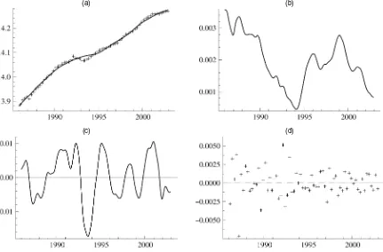
The estimated components for the Euro area real GDP se-ries are presented in Figure 2. Several interesting features be-come apparent. First, although GDP is recorded on a quarterly basis, the estimated components are monthly. These compo-nents can be viewed as the outcome of the underlying monthly GDP decomposition that can be recovered resorting to the infor-mation contained in the remaining dataset. Second, analyzing the trend seems to indicate that Euro area potential growth has declined after the major recession that occurred in 1993. This feature becomes clear by plotting the trend slope against the time axis. Before the 1993 recession, monthly potential growth was around.3% (3.7% in annualized terms), whereas afterward it was closer to.2%. This is 2.4% in annualized terms and falls within the 2.0%–2.5% GDP potential growth range underlying the ECB monetary policy. Third, the resulting GDP cyclical component, our Euro area business cycle indicator, is in line with the common wisdom regarding Euro area business cycle developments (see European Central Bank 2002). In particular, a major recession was recorded in 1993 (as German unifica-tion boost delayed the impact of the recessions in the U.S. and U.K. in the early 1990s) while there was an economic slow-down in the late 1990s after the crisis in Asian emerging market economies and the financial instability in Russia.
(a) (b)
(c) (d)
Figure 2. Decomposition of GDP: (a) GDP and Trend; (b) Slope; (c) Cycle; (d) Irregular.
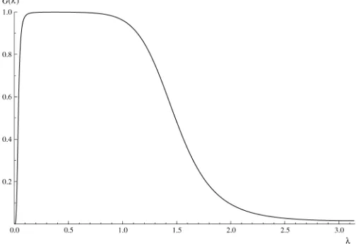
Figure 3. Gain Function of the Implied Univariate Filter for Extracting the Cycle for GDP at a Monthly Frequency. The gain coefficients are from parameter estimates of multivariate model.
The variances of the trends and the damping factor and stan-dard deviation of the common cycle are estimated. For the latter parameters, we obtained estimatesφˆ=.57 andσˆκ=.0066. The
variances of the individual trends are also estimated, and they vary from very small values (suggesting that the trend is fixed and may coincide with the fact that the trend does not exist) to relatively high values (suggesting that trend and its correspond-ing slope change throughout the series).
The estimated business cycle component is computed by the multivariate Kalman filter and smoother, which effectively weight the observations in an optimal way for signal extraction. The associating gain function is also multivariate but is diffi-cult to interpret from a practical standpoint. Therefore, Figure 3 presents the gain function of the univariate filter as given by Harvey and Trimbur (2003, sec. IV). The gain function is for the extraction of the monthly business cycle associated with GDP and is based on coefficients obtained from parameter estimates of the multivariate model. The cutoff at the lower frequencies is sharp, whereas the cutoff at the higher frequencies is more smooth. The latter is due, in part, to the estimateφˆ=.57, be-cause it implies a somewhat less persistent cycle component.
The approach of this article can be viewed as an attempt to extract a business cycle that is similar to that obtained from a filter implied by the gain function of Figure 3 but that is actu-ally based on a dataset of monthly economic indicators, as well as on quarterly GDP. The motivations of this approach are to circumvent the nonavailability of GDP at a monthly frequency and to obtain a clearer signal at the end of the sample. These ob-jectives are important for the policy maker. It should be stressed that Figure 3 gives a distorted picture of the gain function at the end of the sample. However, by using multiple sources of in-formation at a monthly frequency, this distortion is diminished. Furthermore, it may lead to smaller revisions of the signal at the end of the sample when new observations become available.
Some key estimation results are presented in Table 1. It is noted that we do not aim to develop a model that captures all dynamic characteristics in the available panel of time series. Therefore, we do not present a detailed discussion of the esti-mation results for each individual equation of the multivariate
Table 1. Selected Estimation Results
Time series Rel trd Rel cyc Shift RD2
GDP .10 .074 0 .31
Industrial production .068 .064 6.85 .67 Unemployment (inverted sign) .55 .033 −15.9 .78 Industrial confidence .26 .14 7.84 .47 Construction confidence .17 .036 1.86 .51 Retail trade confidence .098 .013 −.22 .67 Consumer confidence .33 .049 3.76 .33 Retail sales .027 .0064 −4.70 .86 Interest rate spread .34 .023 16.8 .22
NOTE: The following values are based on maximum likelihood estimates (denoted by hats):
rel trdmeasures the relative importance of trend component and is computed byσˆi,ζ/(σˆi,ζ+
ˆ
δiσˆκ+ ˆσi,ε);rel cycis for the cycle component and is computed byδˆiσˆκ/(σˆi,ζ+ ˆδiσˆκ+ ˆσi,ε);
shiftreports estimateξˆ
i. The coefficient of determinationR2Dis with respect to the total sum of squared differences.
model. The table aims to provide information about the ade-quacy of our choice of economic variables and their roles in the construction of the multivariate bandpass filter.
The individual time series are decomposed by trend, com-mon cycle, and irregular components. The relative importance of each component for a particular time seriesiis determined by the scalarsσi,ζ (trend),δiσκ(cycle), andσi,ε(irregular).
Ta-ble 1 presents the relative importance of the trend and the cycle based on the maximum likelihood estimates of these scalars. Trend variations appear most prominently in the unemployment series and, to a lesser extent, in the series interest rate spread, consumer confidence, and industrial confidence. It is interest-ing to observe that industrial confidence tops the list of contrib-utors to the construction of the business cycle, whereas GDP, industrial production, consumer confidence, and construction confidence are important as well. Series related to retail trade contribute relatively little to the estimated business cycle.
The ability of simultaneously identifying and estimating cy-cle shifts within the model for a given set of time series is a key development that is important to the current analysis, because it avoids the preselection of coincident variables, whether by lagging or leading the variable. The estimation results reveal that unemployment lags the business cycle by more than 1 year (almost 16 months), whereas interest rate spread clearly leads the business cycle by almost 17 months. The common cycle component for the other series displays relatively small shifts, confirming the coincident character of these series. These re-sults are in line with what was expected and according to what was found elsewhere (see, e.g., Altissimo et al. 2001). An in-dication of whether the multivariate trend-cycle model success-fully fits the individual series is the goodness of fitR2D statistic as reported in Table 1. The sum of squared prediction errors is compared with the sample variance of the differenced time series for each equation of the model. These statistics provide evidence that the model fit for the individual time series is ade-quate to good.
Figure 4 presents the smoothed estimate of the business cy-cle indicator together with the Euro area business cycy-cle turn-ing points settled by the ECB (European Central Bank 2001). Because the ECB dating was done on a quarterly basis, the quar-ters in which a turning point presumably occurred are repre-sented by a shaded area due to the monthly nature of the time axis. One can see that the suggested business cycle indicator generally tracks the turning points quite well. Only at the end
Figure 4. Euro Area Business Cycle Indicator With ECB Datings.
of the sample does it seem to perform less satisfactorily. How-ever, one should note that the ECB dating was done using data only up to 2000. In particular, this can explain why the last peak dated by ECB is not confirmed by our business cycle indicator, because it suggests that the peak occurred only at the beginning of 2001. The historical minimum value of the business cycle is observed in August 1993, which falls within the most severe re-cession period recorded in the Euro area, whereas the maximum value is at January 2001.
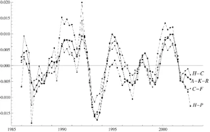
Figure 5 compares the business cycle obtained from our multivariate filter with the ones resulting from some univari-ate approaches to business cycle assessment based on quarterly real GDP. In particular, we consider the Hodrick and Prescott (1997) filter, the Christiano and Fitzgerald (2003) bandpass filter, and the Harvey–Clark model–based filter (Clark 1987;
Harvey 1989). The latter model-based filter is based on the uni-variate trend-cycle decomposition model (1) with N=1. As is standard practice in the literature for quarterly data, we set λ=1,600 for the Hodrick–Prescott filter and considered cycles of periodicity between 6 and 32 quarters for the Christiano– Fitzgerald filter. All cycle indicators appear to move upward or downward at roughly the same time. However, our multi-variate filter provides a smooth business cycle similar to that from Christiano and Fitzgerald (2003) bandpass filter, whereas the other detrending approaches are more affected by irregular movements. The cycle indicators are presented at a quarterly frequency, whereas our multivariate filter obtains business cy-cle estimates at the higher monthly frequency and is able to recover the latent monthly output gap, which is highly relevant for the policy maker. The underlying methods used in this arti-cle also overcome the release lags that end up delaying the as-sessment of the current economic situation and are noteworthy in the Euro area. Because the state-space framework can deal with the missing observations problem, it ensures an up-to-date high-frequency business cycle estimate and allows for a timely analysis of current economic developments.
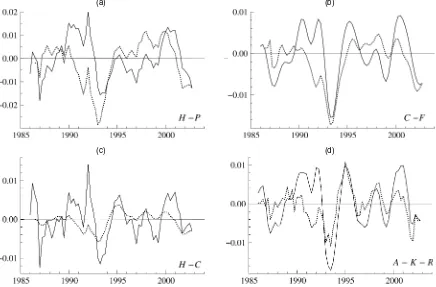
3.4 Revisions
A major issue regarding business cycle estimates is their real-time reliability (see Orphanides and van Norden 2002). In prac-tice, business cycle estimates are subject to revisions over time due to data revision and recomputation when additional data become available. Although it is not possible to evaluate the consequences of the first source of revision for the Euro area due to lack of data vintages, the second source of revision can be assessed by comparing smoothed and filtered estimates of
Figure 5. Comparison of Four Different Business Cycle Indicators: H–P, the Hodrick–Prescott Filter; C–F, the Christiano–Fitzgerald Filter; H–C, the Model-Based Decomposition of Harvey and Clark; and A–K–R, Our Business Cycle Indicator. The business cycle indicators are presented at a quarterly frequency.
(a) (b)
(c) (d)
Figure 6. Comparison of Filtered (· · · ·) and Smoothed ( ——) Estimates Related to Four Different Business Cycle Indicators: (a) H–P, the Hodrick–Prescott Filter; (b) C–F, the Christiano–Fitzgerald Filter; (c) H–C, the Model-Based Decomposition of Harvey and Clark; (d) A–K–R, Our Business Cycle Indicator. The business cycle indicators are presented at a quarterly frequency.
the business cycle. The filtered estimate is the one conditional on the information set available up to each time point, and the smoothed estimate is the one based on the full set of data. Com-paring them reveals the magnitude of the revision. Figure 6 presents final (smoothed) and real-time (filtered) estimates for different filters. In line with the findings of Orphanides and van Norden (2002) for the U.S., the difficulty of assessing the cyclical position in real time for the Euro area is clear. In fact, Orphanides and van Norden (2002) showed that the reliabil-ity of real-time estimates of U.S. output gap is low whatever method is used. In addition to a graphical inspection, the impor-tance of the revisions can be measured by the cross-correlation between final and real-time estimates, by the noise-to-signal ra-tio (the rara-tio of the standard deviara-tion of the revisions to the standard deviation of the final estimate), and by the sign con-cordance (the proportion of time that final and real-time esti-mates share the same sign). These measures are presented in Table 2 for the whole sample and for a more recent period. It
should be borne in mind that it is extremely hard to estimate the output gap in real time, because only with time can one be more accurate about the cyclical position at a given period. Ta-ble 2 shows that the Hodrick–Prescott filter presents the worst results, whereas the multivariate bandpass filter method consid-erably outperforms all univariate filters in real time. Therefore, it seems that a multivariate setting allied with the use of lead-ing, coincident, and lagging variables can overcome to some extent the shortcomings of the currently used filters for real-time analysis.
3.5 A Growth Indicator
The focus of this article is on the business cycle indicator and on how the information content of an economy-wide dataset can be exploited for the assessment of the cyclical position of the economy using a multivariate approximate bandpass filter. Nevertheless, a policy maker may also be interested in tracking
Table 2. Reliability Statistics for Different Business Cycle Indicators
Correlation Noise-to-signal Sign concordance
Method 86–02 93–02 86–02 93–02 86–02 93–02
Hodrick–Prescott .33 .70 1.23 .99 .47 .55 Christiano–Fitzgerald .54 .76 .90 .67 .55 .65
Harvey–Clark .42 .69 .91 .75 .61 .63
Azevedo–Koopman–Rua .58 .80 .81 .61 .69 .83
NOTE: Correlation is the contemporaneous correlation between the real time (filtered) estimates and the final (smoothed) es-timates of the business cycle. Noise-to-signal ratio is the ratio of the standard deviation of the revisions against the standard deviation of the final estimates. Sign concordance is the percentage of time that the sign of the real time and final estimates are equal. The statistics are reported for the sample periods of 1986–2002 (86–02) and 1993–2002 (93–02).
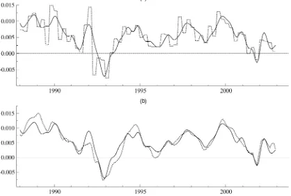
(a)
(b)
Figure 7. Comparisons of (a) Euro Area Quarterly GDP Growth (· · · ·) versus Our Growth Indicator ( ——) and (b) EuroCOIN Indicator (· · · ·) versus Our Growth Indicator ( ——).
economic activity growth. As a byproduct, a growth indicator can be obtained as part of our model-based approach. This can be done by restoring the smoothed estimate of the business cy-cle together with the corresponding smoothed estimate of the trend component of a particular time series and by comput-ing its growth rate. The 3-month change of the trend restored business cycle indicator is presented in Figure 7. The resulting growth indicator can be interpreted as the latent monthly mea-sure of GDP quarterly growth. Figure 7 shows that the growth indicator tracks GDP quarterly growth quite well. Moreover, it is available on a monthly basis and avoids the erratic behavior of GDP quarterly growth rate that complicates the assessment of the current economic situation. Figure 7 also presents our growth indicator together with EuroCOIN (see Altissimo et al. 2001). EuroCOIN is based on the generalized dynamic factor model of Forni et al. (2000) and resorts to a huge dataset (almost 1,000 series that refer to the six major Euro area countries). The model underlying EuroCOIN can be briefly described in the fol-lowing way. Each series in the dataset is modeled as the sum of two uncorrelated components, the common and the idiosyn-cratic. The common component is driven by a small number of factors common to all variables but possibly loaded with differ-ent lag structures, whereas the idiosyncratic compondiffer-ent is spe-cific to each variable. EuroCOIN is the common component of the GDP growth rate after discarding its high-frequency com-ponent. The EuroCOIN indicator presented in Figure 7(b) has been subject to revisions each time that new observations be-come available. Note that the GDP monthly series used as in-put was obtained through the linear interpolation of quarterly figures. Although this approach allows for more general
cycli-cal dynamics compared with our model, it has additional draw-backs. For instance, it requires detrending of the series prior to dynamic factor analysis and series of different periodicities cannot be used simultaneously. Moreover, with the estimation of only two parameters for each series, the common cycle fac-tor load, and the shift, we are able to get a quite similar out-come.
4. CONCLUSION
In this article we propose a multivariate approximate band-pass filter for obtaining a business cycle indicator. The filter is based on a multivariate unobserved components time series model that incorporates two recent and relevant contributions: (a) the inclusion of a particular cycle component that has prop-erties similar to those of bandpass filtered series (see Harvey and Trimbur 2003) and (b) the incorporation of phase shifts within the cycle component (see Rünstler 2004). The result-ing multivariate filter is used to extract trend and cycle com-ponents using several economic time series for the Euro area. The innovations to the cycle component of each time series are common, but their contribution is derived from a model-based filter that depends only on three parameters. One pa-rameter is the frequency of the cycle, which we fix so as to ensure that the typical business cycle frequencies are captured. Another parameter accounts for phase shifts, whereas the third parameter accounts for the relative contribution of the cycle to the dynamics of the individual time series. The common cycle component resumes to our business cycle indicator. These gen-eralizations lead to a smooth business cycle indicator, and the
suggested procedure can be viewed as a multivariate bandpass filter. Besides the multivariate setting, we are not constrained to use only coincident variables to identify the business cycle, as done by Stock and Watson (1989), because we account simul-taneously for phase shifts between the cyclical components of the series. Thus one can also exploit the information contained in both leading and lagging variables, which allows for a richer information set when obtaining the business cycle. This multi-variate approach is shown to provide business cycle estimates that are less subject to revisions than those resulting from the commonly used filters. This feature represents a valuable im-provement for policymaking, because reliable estimates of the current cyclical position are required in real time when policy decisions are made. Moreover, we are also able to reconcile in-formation available at different frequencies. It becomes possi-ble to obtain a high-frequency business cycle indicator without discarding series such as GDP despite its quarterly frequency, as done by Stock and Watson (1989). The use of quarterly GDP together with monthly indicators can be dealt with straightfor-wardly by exploiting the state-space framework in a consistent manner. Furthermore, the ability to deal with missing obser-vations also allows timely business cycle estimates regardless of data release lags, which can be substantial in the Euro area. This feature is also crucial for the policymaker because it per-mits an evaluation of the current state of the economy without delay. The new approach is applied to Euro area data, and the re-sulting business cycle indicator appears to be in line with com-mon wisdom regarding Euro area economic developments. As a byproduct, one can also obtain a growth indicator. In particu-lar, our more parsimonious approach leads to a growth indicator for the Euro area similar to EuroCOIN. The latter is based on a more involved approach by any standard and uses hundreds of time series from individual countries belonging to the Euro area. Furthermore, the suggested procedure of this article also overcomes some of the drawbacks of the EuroCOIN procedure.
APPENDIX A: PHASE SHIFTS FOR THE GENERALIZED CYCLE
The cycle shifts are modeled as shifts in the cross-autocovari-ance function for different cycles. In the common cycle compo-nent model (1), (3), and (4), the cross-autocovariance function for the cycle component is given by
γij(τ )=E(ψitψj,t−τ)
=σκ2φτ(1−φ2)−1δiδjcos{λ(τ+ξi−ξj)},
i,j=1, . . . ,N, (A.1)
forτ =0,1, . . . ,where
ψit=δi{cos(ξiλ)ψt+sin(ξiλ)ψt+}, t=1, . . . ,n,
with ψt modeled by (4). This result is a direct consequence
of the general results given by Rünstler (2004, prop. 1). The contemporaneous correlation between elements i andj inψt
is γij(0)/ γii(0)γjj(0)=cos{λ(ξi−ξj)}. However, when
cy-cles are shifted accordingly, the correlation is cos(0)=1, as expected from a common cycle specification. It is important to realize that a real-time shiftξi is rarely estimated as an
in-teger time point, and because observed time series data can
be shifted only at discrete time intervals, the contemporaneous cross-correlation of cycles associated with shifted time series will usually be smaller than 1.
The autocovariance function of the generalized cycle (8) is reported as the proof of prop. 2). The cross-autocovariance function of the generalized shifted cycle component is then given by
γij(τ )=σκ2φτδiδjcos{λ(τ+ξi−ξj)}g(φ, τ ), (A.3)
forτ=0,1,2, . . .. This result follows straightforwardly by ap-plying proposition 1 of Rünstler (2004) to the proof of proposi-tion 2 of Trimbur (2002). Because the autocovariance funcproposi-tion for generalized cycles also applies to negative discrete values forτ and is symmetric inτ =0, the shift mechanism has the desired effect on the autocovariance function of the shifted cy-cle.
It follows that the shift mechanism of Rünstler (2004) can also be applied to correlated generalized cycles whether or not the correlation is perfect. This means that cycles with bandpass filter properties can be subject to shifts within a multivariate cy-cle model based on the generalized cycy-cle component (8). In the case of model (9), the properties of the cycle component for the first series in the panel will be closely related to those of the uni-variate bandpass-filtered series. However, the information from the other series is also exploited in the estimation of the cycle component.
APPENDIX B: STATE–SPACE REPRESENTATION OF THE MODEL
A state-space representation consists of two equations, the observation equation for yt and the transition equation that
describes the dynamic process through the state vector. The model (9) requires the following state vector:
αt= linear combination of the state together with observation noise, that is,
yit= {ei 01×(m−1)N δicos(λξi) δisin(λξi) 01×2(k−1)}αt
+εit, i=1, . . . ,N,
whereei is the ith row of the N×N identity matrix IN and
0p×qis thep×qmatrix of 0’s.
DefineApas ap×p matrix with zero elements except for
elements(i,i+1), which are equal to unity fori=1, . . . ,p−1. The transition equation for the state vector is then given by
αt+1= agonal matrix. The initial state vectorαµ1 is treated as a fully diffuse vector and appropriate amendments to the Kalman filter and related algorithms must be made (see Durbin and Koopman 2001, chap. 4, for a discussion). The stochastic properties of the initial state vectorαψ1 are implied by mean vector0and vari-ance matrixP, which is the solution of
P= [Ik⊗Tλ+Ak⊗I2]P[Ik⊗Tλ+Ak⊗I2]′
+diag[02(k−1)×2(k−1) σκ2I2]. We note that the solution ofA=BAB′+Cis vec(A)=(I− B⊗B)−1vec(C)(see Magnus and Neudecker 1988, thm. 2, p. 30). Explicit formulations forPhave been given by Trimbur (2002).
The multivariate state-space model under consideration is linear and Gaussian. Standard Kalman filter and smoothing techniques thus can be used for maximum likelihood estimation and signal extraction. The computational effort for a multivari-ate model can be severe when the dimension of the observation vector N is relatively large; however, the computational load can be reduced considerably when the elements of the observa-tion vectorytare treated element by element when filtering and
smoothing updates are carried out at each time pointt. Because the irregular variance matrix is diagonal, we can adopt this approach straightforwardly (see Durbin and Koopman 2001, sec. 6.4). The actual reduction of computing time in our case has been in the neighborhood of 50%.
All computations for this article are done using the object-oriented matrix languageOxof Doornik (2001) together with the state-space functions in version 3 ofSsfPackas developed by Koopman, Shepard, and Doornik (1999) (for later versions, seehttp://www.ssfpack.com).
APPENDIX C: DATA DETAILS
As far as possible, we used series from Euro area official sta-tistical sources (i.e., Eurostat), the European Commission, and
the ECB. However, the available data regarding the Euro area as a whole is rather limited, particularly in terms of time span. Therefore, in some cases we had to chain the official time se-ries with an Euro area aggregate proxy, obtained by weighting country-level data with 1995 (PPP) GDP weights, which were rescaled whenever there were any missing data for a country. The sample runs from the beginning of 1986 up to the end of 2002. Regarding real GDP, the seasonally adjusted series pro-vided by the Eurostat starts only in the first quarter of 1991. Therefore, from 1991 backward, we used the series provided by Fagan, Henry, and Mestre (2001) to obtain a quarterly se-ries for the afore mentioned sample period. All confidence in-dicators are seasonally adjusted and provided by the European Commission. The industrial production volume index is season-ally adjusted and provided by the Eurostat. The unemployment level series is also seasonally adjusted and provided by the Eu-rostat. Because there is no official series before June 1991, an aggregate series was obtained in this particular case by sum-ming country-level data. The retail sales volume index is sea-sonally adjusted and provided by the Eurostat since 1996. To obtain a longer time span series, we resorted to country-level data provided by the OECD. Regarding nominal interest rates, because both short and long-term interest rates are made avail-able by the ECB only for the period after January 1994, we had to also use OECD country-level data. The nominal short-term interest rate refers to the 3-month deposit money market rate, and the nominal long-term interest rate refers to the 10-year government bond yield. The yield curve spread is given by the difference between the long-term and the short-term interest rates. Excluding confidence indicators and interest rate spread, all data are in logarithms.
[Received November 2004. Revised August 2005.]
REFERENCES
Ahn, S. K., and Reinsel, G. C. (1988), “Nested Reduced-Rank Autoregressive Models for Multiple Time Series,”Journal of the American Statistical Asso-ciation, 83, 849–856.
Altissimo, F., Bassanetti, A., Cristadoro, R., Forni, M., Lippi, M., Reichlin, L., and Veronese, G. (2001), “EuroCOIN: A Real-Time Coincident Indicator of the Euro Area Business Cycle,” Working Paper 3108, CEPR, London. Baxter, M., and King, R. (1999), “Measuring Business Cycles: Approximate
Band-Pass Filters for Economic Time Series,”Review of Economics and Sta-tistics, 81, 575–593.
Christiano, L., and Fitzgerald, T. (2003), “The Band-Pass Filter,”International Economic Review, 44, 435–465.
Clark, P. K. (1987), “The Cyclical Component of U.S. Economic Activity,”The Quarterly Journal of Economics, 102, 797–814.
Doornik, J. A. (2001),Object-Oriented Matrix Programming Using Ox 3.0
(4th ed.), London: Timberlake Consultants,http://www.doornik.com. Durbin, J., and Koopman, S. J. (2001),Time Series Analysis by State-Space
Methods, Oxford, U.K.: Oxford University Press.
Engle, R. F., and Kozicki, S. (1993), “Testing for Common Features” (with discussion),Journal of Business & Economic Statistics, 11, 369–395. European Central Bank (2001), “The Information Content of Composite
In-dicators of the Euro Area Business Cycle,” Monthly Bulletin, November, pp. 39–50.
(2002), “Characteristics of the Euro Area Business Cycle in the 1990s,” Monthly Bulletin, July, pp. 39–49.
Fagan, G., Henry, J., and Mestre, R. (2001), “An Area Wide Model for the Euro Area,” Working Paper 42, European Central Bank, Frankfurt.
Forni, M., Hallin, M., Lippi, M., and Reichlin, L. (2000), “The Generalized Factor Model: Identification and Estimation,”Review of Economics and Sta-tistics, 82, 540–554.
Gomez, V. (2001), “The Use of Butterworth Filters for Trend and Cycle Estima-tion in Economic Time Series,”Journal of Business & Economic Statistics, 19, 365–373.
Harvey, A. C. (1989),Forecasting, Structural Time Series Models and the Kalman Filter, Cambridge, U.K.: Cambridge University Press.
(1993),Time Series Models(2nd ed.), Hemel Hempstead: Harvester Wheatsheaf.
Harvey, A. C., and Jaeger, A. (1993), “Detrending, Stylised Facts and the Busi-ness Cycle,”Journal of Applied Econometrics, 8, 231–247.
Harvey, A. C., and Koopman, S. J. (1997), “Multivariate Structural Time Series Models,” inSystematic Dynamics in Economic and Financial Models, eds. C. Heij, H. Schumacher, B. Hanzon, and C. Praagman, Chichester, U.K.: Wiley, pp. 269–298.
(2000), “Signal Extraction and the Formulation of Unobserved Com-ponents Models,”Econometrics Journal, 3, 84–107.
Harvey, A. C., and Trimbur, T. (2003), “Generalised Model-Based Filters for Extracting Trends and Cycles in Economic Time Series,”Review of Eco-nomics and Statistics, 85, 244–255.
Hodrick, R. J., and Prescott, E. C. (1997), “Postwar U.S. Business Cycles: An Empirical Investigation,”Journal of Money, Credit and Banking, 29, 1–16. Koopman, S. J., and Durbin, J. (2000), “Fast Filtering and Smoothing for
Mul-tivariate State-Space Models,”Journal of Time Series Analysis, 21, 281–296. Koopman, S. J., Shephard, N., and Doornik, J. A. (1999), “Statistical Algo-rithms for Models in State-Space Form Using SsfPack 2.2,”Econometrics Journal, 2, 113–166.
Magnus, J. R., and Neudecker, H. (1988),Matrix Differential Calculus With Applications in Statistics and Econometrics, New York: Wiley.
Mariano, R. S., and Murasawa, Y. (2003), “A New Coincident Index of Busi-ness Cycles Based on Monthly and Quarterly Series,”Journal of Applied Econometrics, 18, 427–443.
Orphanides, A., and van Norden, S. (2002), “The Unreliability of Output-Gap Estimates in Real Time,”Review of Economics and Statistics, 84, 569–583. Rünstler, G. (2004), “Modelling Phase Shifts Among Stochastic Cycles,”
Econometrics Journal, 7, 232–248.
Stock, J., and Watson, M. W. (1989), “New Indexes of Coincident and Leading Economic Indicators,” Macroeconomics Annual 1989, National Bureau of Economic Research.
(1999), “Business Cycle Fluctuations in U.S. Macroeconomic Time Series,” inHandbook of Macroeconomics, eds. J. B. Taylor and M. Wood-ford, Amsterdam: Elsevier Science, pp. 3–64.
(2002), “Macroeconomic Forecasting Using Diffusion Indexes,” Jour-nal of Business & Economic Statistics, 20, 147–162.
Tiao, G. C., and Tsay, R. S. (1985), “A Canonical Correlation Approach to Modeling Multivariate Time Series,” inProceedings of the Business and Eco-nomic Statistics Section, American Statistical Association.
Trimbur, T. (2002), “Properties of a General Class of Stochastic Cycles,” mimeo, University of Cambridge.
![Figure 1. Nine Key Economic Variables for the Euro Area, 1986–2002 [GDP;fidence indicator;IPI;interest rate spread;construction con-consumer confidence indicator;retail sales;unemployment (inverted sign);industrial confidence indicator;retail trade confidence indicator].](https://thumb-ap.123doks.com/thumbv2/123dok/1120821.760964/6.594.85.489.42.310/variables-construction-condence-indicator-unemployment-industrial-condence-condence.webp)