Review article UDC: 332.74:332.821(510) doi: 10.10.18045/zbefri.2015.2.325
Heterogeneous convergence of regional house
prices and the complexity in China
*1Rui Lin
2, Xin Zhang
3, Xiuting Li
4, Jichang Dong
5 AbstractThe purpose of this research is to analyze the convergence of regional house prices and its complexity in China. In this purpose it used nonlinear time varying factor model. The obtained results have provided evidences for the existence of some degree of segmentation in China’s housing market. By further dynamic analysis of the convergence, we have found that important housing policies from Chinese central government can significantly alter the housing market but with a time lag of 4 to 5 months, and that quite different behaviors exist between the new house market and the second-hand house market in China, which provides the evidence for the complexity of housing market in China. Multiple factors together are the driving forces for the regional house price convergence. And the driving forces differ among three clubs. The basic conclusion provided from the realized research is that the conventional definitions of economic regions may not be appropriate to
* Received: 22-09-2015; accepted: 15-12-2015
1 This work was supported by the National Natural Science Foundation of China under Grant No. 71173213; the National Natural Science Foundation of China under Grant No. 71203217; 71403260 and the China Postdoctoral Science Foundation under Grant No. 2013M540129. 2 PhD, School of Economics and Management, University of Chinese Academy of Sciences, Beijing
100190, China, Department of Sociology, University of Chicago, 5801 S Ellis Ave, Chicago, IL 60637, USA. Scientific affiliation: real estate economics. Phone: +86 1 5201 305 859. E-mail: linrui0704@163.com. Website: http://www.mscas.ac.cn/.
3 PhD, School of Economics and Management, University of Chinese Academy of Sciences, Beijing 100190, China. Scientific affiliation: real estate economics. Phone: +86 18810404354. E-mail: zhangxin2970@163.com. Website: http://www.mscas.ac.cn/.
4 Assistant Professor, School of Economics and Management, University of Chinese Academy of Sciences, Beijing 100190, China. Scientific affiliation: real estate economics, behavioral finance. Phone: +86 1 3811 580 462. E-mail: lixiuting@ucas.ac.cn. Website: http://www.mscas.ac.cn/ Teachers/Professor/243.shtml. (corresponding author).
5 Full Professor, School of Economics and Management, University of Chinese Academy of Sciences, Beijing 100190, China. Scientific affiliation: real estate economics, financial engineering. Phone: +86 1 3521 211 972. E-mail: jcdonglc@ucas.ac.cn. Website: http://www. mscas.ac.cn/Teachers/Professor/201.shtml.
analyze house price segregation in China. Heterogeneous convergence exists in China’s regional house prices, indicating the complexity of regional house prices in China. And housing policies should be implemented with different focus among the regions. The way of the central government is to make housing policies aiming at different sub-markets of the new house market and the second-hand house market.
Key words: convergence, house prices, China; policy, complexity JEL classification:E30, P25, R11
1. Introduction
China has been undergoing a rapid growth in its housing market as well as its economy over the recent decade. However, the house prices have been increasing so fast that the Chinese government has to implement a series of policies and regulations to control them especially since the end of 2009. In April 2010, the
State Council of the PRC started the first-round control with a notice of “Firmly
Curbing the Surge in House price in Some Cities” (also known as No. 10 National
Notice) which was claimed as a “most severe” policy of control over the housing
market. Since then, a bunch of other policies and regulations on China’s housing market have been issued. In this regard, it is of great importance to explore the growth ways of house prices across regions in China and how they are affected by those control policies.
Following Kim et al. (2012) and Montañés et al. (2013), in this paper, we have employed a relatively new convergence methodology by Phillips and Sul (2007, 2009) rather than the conventional way of using unit root tests to analyze the convergence of house prices in China, because failing to reject the unit root null hypothesis does not necessarily imply the absence of convergence. By taking advantages of the new method which allows for a wide range of transitional dynamics and individual heterogeneity, the hypothesis of this research is to examine empirically whether there is a single common convergence factor or otherwise possible segmentation across regions in China’s housing market.
The rest of this paper is organized as follows. Section 2 reviews the literature and the results concerned with the problem of convergence of house prices and describes the heterogeneity of regional house prices qualitatively. Section 3 introduces the relative convergence and log t convergence test, and the Club Convergence and Clustering procedure. Section 4 describes the data, presents the
results and discusses the implications of our findings. Section 5 explores the driving forces for the regional house price convergence. In the final section, a review of all
2. Literature review
As for the problem of convergence of house prices, researchers in the UK and
the USA seem to be playing a leading role, and some important results have been obtained. These include evidences for a certain degree of segmentation in both
the housing markets of the UK (MacDonald and Taylor, 1993; Cook, 2003) and
the USA (Gabriel, 1989; Haurin, 1996; Meen, 2002; Downes, 2002; Gallin, 2006;
Hwang, 2006; Kiel, 2008; Mikhed, 2009; Montañés, 2013; Miles, 2015), the influences of the east and west coast metropolitan areas (Canarella et al., 2012) and the bursting of the house price bubble (Montañés, 2013) on the housing market in the USA, etc.
However, very few studies have aimed at China’s housing market except for one by Herrerias (2012) which indicates that Chinese regions have converged into
clubs. While, Fang Zhang and Bruce Morley (2014) show little evidence for
convergence across the regions in China. Most of the previous studies focus on the empirical analysis of regional difference of Chinese house prices, based on
the traditional definition of economic regions and administrative regions. For
instance, some researchers analyzed the difference of house price among the West, the East and the Central regions in China (Chen and Wang, 2000). And there are also studies that analyzed the features of regional house prices among
economic regions including Huanbohai region (Zhang, 2011), the Yangtze River Delta (Wei and Yang, 2007) and the Pearl River Delta (Chen and Huang, 2010), etc. Few researchers have examined empirically whether there is a single common
convergence factor or otherwise possible segmentation across regions in China’s housing market.
The methodologies commonly used in previous studies on convergence of
house prices can mainly be summarized into three categories. The first category
is unit root test and its various extended forms including panel data unit root testing and unit root testing with structure breaks (Clark and Coggin, 2009), etc. The disadvantage of unit root tests is that it does not necessarily imply the existence of convergence when the unit root test cannot be rejected (Montañés and Olmos, 2013).The second category is Granger causality test combined with VAR models, cointegration test and impulse response, etc. (Cooper et.al. 2013).
The disadvantage of these methods is about the DOF constraints for these models
can’t contain too much regional units (typically less than 8). The third category is spatial or temporal models (Gupta and Miller, 2012). These models have to be
set based on spatial weights matrix, which is generally defined by “geographical adjacent” or “economic proximity”. And the selection of spatial weight matrix
3. Methodology and conception of analysis
3.1. The relative convergence and log t convergence test
The reason why the convergence method by Phillips and Sul (2007, 2009) is employed in this paper concerns two aspects. One is that traditional unit root tests,
such as the ADF and PP unit root tests, suffer from over-rejection of the unit-root
hypothesis (Ng & Perron, 2001). Second is that the time series approach cannot deal with individual heterogeneity and so a panel approach is preferred. The panel data model by Phillips and Sul (2007, 2009) not only takes into account the heterogeneity of individuals, but also allows regional clusters to be tested for. Actually, these features of the model are very suitable to study the regional house prices of China. In the last four decades, Chinese economy has gone through
the reform and opening-up, and has been undergoing a process of significant
transformation. The effect on technological and capital accumulation caused by the different economic policies introduced by the Chinese government usually
benefit some provinces, often located on the coast, at the expense of other inland
regions. China’s regional house prices most likely have different speeds of convergence under such circumstances. The house price of different regions in China with different economic sizes and populations may appear to follow a similar development path but at different speeds, so that they are currently at different
stages on that path. Fortunately, these idiosyncratic behaviors can be captured by
the time-varying nature of the model.
Generally, the panel data Xit can be decomposed into two parts as follows.
Xit = git + a (1)
Where git embodies systematic components, including permanent components that give rise to cross section dependence, and ait represents transitory component. Continue to transform Eq. (1) as follows:
( it it) it t it t t g a X µ δ µ µ +
= = for all i and t (2)
Where μt is a single common component and δit is a time varying idiosyncratic one. A semiparametric model for the time-varying behavior of δit is proposed as follows:
δit = σiξitL(t)–1t–α (3)
Where δi is fixed, σi > 0, ξit is i.i.d (0,1) across i but weakly dependent on t, and
L(t) is a slowly varying function for which L(t) → ∞ as t → ∞. The L(t) function is assumed to be log t by following Phillips and Sul (2007). ξit introduces time-varying and region-specific components to the model. The size of α determines the
behavior (convergence or divergence) of δit. This formulation ensures convergence of the parameter for all α ≥ 0, which is the null hypothesis of interest since δit = δi as t → ∞. Furthermore, if this hypothesis holds and δi = δj for i ≠ j, the specification in Eq. (3) still allows for transitional periods in which δit ≠ δjt, thereby incorporating the interesting possibility of transitional heterogeneity or even transitional divergence across i.
Thus, the null hypothesis of convergence can be written as:
H0: δit = δandαi ≥ 0 (4)
and the alternative HA: δit ≠ δfor all ior α < 0.
The null hypothesis H0 can be tested as the following three steps:
Step 1: Construct the cross-sectional variance ratio H1/Ht, where
1 2 1 ( 1) N t it i H N− h = =
∑
− , 1 1 it it N it i X h N− X = =∑
(5)The variable hit is called the relative transition path which traces out an individual trajectory for each i relative to the panel average. When there is a common limiting transition behavior across regions, hit = ht for all i. When there is ultimate growth convergence, then hit → 1 for all i as t → ∞.
Step 2: Run the following regression and compute a conventional robust t statistic,
tbˆ, for the coefficient bˆ using an estimate of the long run variance of the regression residuals:
1
log( ) 2log(log( )) log t
t
H t a b t u
H − = + + , for t = [rT], [rT] + 1,…, T with r > 0. (6) The key parameter of the convergence test b is related with α (bˆ = 2αˆ) where αˆ is the estimated value of α under the null. In this method, rejection of the null for the whole panel does not imply that there is not convergence, since it is possible to test, by means of an algorithm, whether there are clubs/clusters of convergence. Hence, it is possible to test the hypothesis of convergence for different groups of countries, and identify commonalities within a panel of countries. Phillips and Sul (2007) suggested r = 0.3 based on their simulation experiments.
Step 3: Apply an autocorrelation and heteroskedasticity robust one-sided t test of the inequality null hypothesis α ≥ 0 using the estimated coefficient bˆ and HAC standard errors. At the 5% level, the null hypothesis of convergence is rejected if the statistic has a value below -1.65.
3.2. Club convergence and clustering
As pointed out by Phillips and Sul (2007), the rejection of the null of convergence does not necessarily imply divergence, because there may exist subconvergent clubs. In this regard, Phillips and Sul (2007) suggested the following steps to achieve the possible subconvergent clubs.
In the first step, all the individuals in the panel should be ordered according to the last observation in the panel. The second step is to form a “core group” by running
the log t regression and calculating the convergence test statistic tk(Gk) repeatedly. Firstly select the first k highest individuals in the panel to form the subgroup Gk (2 ≤ k < N), and then run the log t regression to obtain the convergence test statistic
tk(Gk) for this subgroup. The core group size k* is actually chosen by maximizing tk over k according to the following criterion:
k* = arg max
k {tk}, s. t. min {tk} > –1.65. (7)
The latter condition min {tk} > –1.65 is to ensure that the null hypothesis of convergence is supported for each k. Meanwhile, k* = arg max
k {tk} could help to reduce the overall type II error probability for each k and ensure the core group Gk to be a convergence subgroup with a very low false inclusion rate. If there is only a single convergence club with all the regions belonging to the same group, the size of the club is N. In contrast, there are two or more convergence clubs with the membership less than N for each club. If the condition min {tk} > –1.65 is not met for k = 2, the highest individual in Gk have to be dropped from each subgroup and new subgroups G2j = {2, ..., j} will be created for 2 ≤ j ≤ N. The above process will be repeated as many times as necessary until the criterion is satisfied. There could
be no convergence subgroups in the panel if the criterion does not hold for all such
sequential pairs. Otherwise, we could find a core convergence subgroup called Gk*. In the third step, we will add more members to the core group Gk* from the complementary set of Gk*. Denote the complementary set of Gk* to be Gck*. Add one individual in Gc
k* at a time to the original Gk*and run the log t test. If the t statistic of the log t test is big than c, where c is some chosen critical value, include the individual in the convergence club, or not. Basically the critical value c is set to be zero. Repeat this procedure for all the remaining individuals in Gc
k*, and thereafter form the first subconvergence club. To make sure tbˆ > –1.65 for the whole club, run the log t test with this first club. If tbˆ ≤ –1.65, raise the critical value c until
tbˆ > –1.65.
The last step is to deal with the remaining individuals in Gc
k* after the third step, and can be a stopping rule. Treat all the remaining individuals in Gc
k* after the third step as a subgroup, and run the log t test for this subgroup. If tbˆ > –1.65, this subgroup converges. Thus there are only two convergent clubs in the panel. If not,
a smaller subgroup. If there is no k in the second step for which tk > –1.65, it can be concluded that the remaining individuals are divergent.
4.
Empirical data and analysis
4.1. Data
The data used in this paper have been obtained from the official database of the
National Bureau of Statistics of the PRC (NBSC, and Wind database. Three house-price indicators have been selected for this paper: (1) the average sales house house-prices for the 31 regions of Mainland China (ASHP)6, (2) the Sales Price Indices of Newly
Constructed Commercial Residential Buildings (affordable housing excluded) in 70 Large and Medium-Sized Cities (SPI-N, Chain Index: previous month = 100) and (3) the Sales Price Indices of Second-Hand Residential Buildings in 70 Large and Medium-Sized Cities (SPI-S, Chain Index: previous month = 100). Due to the
availability of the information, 30 areas (Tibet excluded) are finally considered for the first indicator (ASHP) with the common sample covering the period 2001:M1-2013:M12 (156 observations), while 69 Large and Medium-Sized Cities (Yangzhou
excluded) are considered for the latter two (SPI-N & SPI-S) with the common
sample covering the period 2005:M7-2014:M2 (104 observations). For all of the
three indicators, some separate missing data are interpolated by using the method of Catmull-Rom Spline7 (Catmull and Rom, 1974). Since all the raw values of the
latter two indicators (SPI-N & SPI-S) are based on “the previous month = 100”, we have adjusted them to be based on the first observations (2005:M7) so as to match the convergence model. Given that the use of seasonal filters may change the time
properties of the variables (Ghysels and Perron, 1993), we prefer to use the non-seasonally-adjusted monthly indicators for all of the three, following Montañé et al. (2013).
Besides, seven indicators are used in regression model to explore the driving forces of the convergence. Considering the data accessibility, we choose GDP growth rate, purchased land area in current year, per capita disposable income of urban residents, domestic loans for real estate development, built-up area and one-lagged
house price as the proxy variables for economic fluctuation level, land supply, urban
residents’ income, credit scale of real estate development, city size and house price
6 Since the NBSC does not provide such an indicator directly, the ASHP is computed by year-to-date
total housing sales divided by year-to-date total housing sales area. Besides, to dissipate the impact of the inflation, the ASHP is further divided by the fixed base CPI (2001M1=100), and multiplied by 100 to keep its data scale.
7 By the Catmull-Rom spline, the interpolated value is usually calculated by two previous values and
two next values. In this paper, when there is no previous value, we just simply set the previous value equal to the unknown value which is going to be interpolated for the calculation.
expectation respectively. And variables related to price are real values eliminated
effects of inflation as before. The data used is annual data span from the year 1999
to 2013.
4.2. Convergence tests and results
To get an intuitive learning of the heterogeneity before convergence tests of
regional house prices in China, we firstly look at the house prices (the house price =
house sales / house sales areas) of 30 regions8 with the data covering from 2001:M1
to 2013:M12. Some missing data is obtained by using the Catmull-Rom spline interpolation9, and the effects of inflation10 for all data are removed.
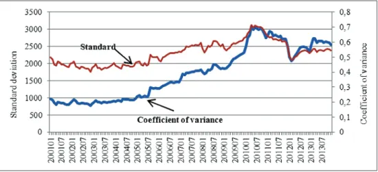
Figure 1 demonstrates the trends of the standard deviation and the coefficient of variance of the house prices of 30 regions. As shown, in the first 10 years of the observed sample period, both of the standard deviation and the coefficient of
variance keep increasing, which means that the discrete extent of regional house
prices is increasing. For this phenomenon, it could be understood that the regional
house prices are divergent, so the differences among some regional house prices are expanding. It could also be understood as another situation, namely regional house prices are heterogeneous convergence. Different regional house prices converge into different groups. Under such situation, both of the standard deviation and the
coefficient of variance of regional house prices could also keep increasing. In either case, the increasing trends of the standard deviation and the coefficient of variation of regional house prices in the first 10 years provide evidence for the regional
differences of regional house prices. After the year of 2010, both of the standard
deviation and the coefficient of variation of regional house prices tend to decrease.
Recalling that 2010 is the beginning year of China's real estate macro-control to be stronger and stronger, it could be inferred that the growths of regional house prices
are affected significantly by the real estate macro-control. This inference will be verified in the later part of this paper.
8 Because of the availability of the data, the sample does not include Tibet, Hongkong, Macao and
Taiwan.
9 The method of Catmull-Rom spline interpolation generally calculate the missing data by the former
two data and the latter two data of the missing data. In this paper, for the missing data without previ-ous data, we assume that the former two data equal to the missing data, then calculate the missing data by the formula of Catmull-Rom spline interpolation.
10 Steps to remove the effects of inflation: (1) Calculated the new values of CPI with the CPI value of
January, 2001 as the base value (2001M1=100); (2) Divide the house prices of all the regions by the new CPI values to obtain the real house prices of all regions.
Figure 1: Standard deviation (left) and coefficient of variance (right) of house prices
for 30 regions
Source: National Bureau of Statistics of the PRC (NBSC, http://www.stats.gov.cn/)
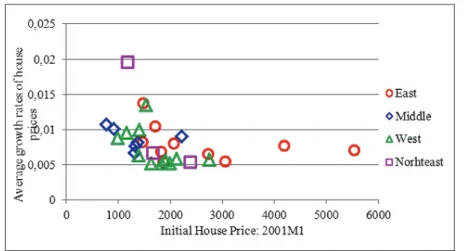
Figure 2 reflects the initial house price level and the average growth rate of the
30 regions within observed sample period, and marks the categories in accordance with the east, middle, west and northeast. The horizon axis represents the values of regional house prices in the initial period (2001:M1), while the vertical axis represents the regional average growth rate of regional house prices during the
period of 2001:M1 to 2013:M12. As shown in Figure 2, the average growth rate
may vary greatly even with the same initial regional house price level. Which means that there may exist quite different growing (or convergent) ways among these regions. Similarly, the initial regional house price level may also vary greatly with similar average growth rates, which means the future growth mode of regional house prices cannot simply be predicted by the initial house price level. Therefore, the current category for regional house prices by different house price level, such
as first-tier cities, second-tier cities and three & four-tier cities, may not be suitable
for the regional differentiated real estate regulation. In addition, through the marks
according to the east, the middle, the west and the northeast in Figure 2, we can see
the mutual penetration and overlap among the different regions, which obviously mean that the traditional way of categorizing should not be used as the guidance of implementing the regional differentiated real estate regulation. It will also be
Figure 2: Average growth rates of house prices for 30 regions: 2001M1-2013M12
Source: National Bureau of Statistics of the PRC (NBSC, http://www.stats.gov.cn/)
Next we take the first observation of the ASHP as the base year (value = 100) and
process the data logarithmically by rewriting it as log Pit = log(P0it/P01t), where P0it is the value of the ASHP of the i-th area at time t, following Phillips and Sul (2007,
2009). Then we smooth the ASHP by the HP filter (Hodrick and Prescott, 1997) to
separate out the cycle. Some initial observations (about 38%) have been discarded to avoid the base year effects from the base year initialization. Consequently, the effective sample size covers the period 2006:M1-2013:M12. The estimation of the log-t coefficient for the ASHP is -0.392 with its corresponding t-ratio -30.208, which implies that the null hypothesis of convergence could be easily rejected even at the
1% significance level. To further examine any possible overall convergence across
regions in China, we divide the housing markets into two sub-markets, i.e. the new house market and the second-hand house market, and run the convergence tests11
again for the SPI-N (log-t: -0.636; t-ratio: -19.801) and the SPI-S (log-t: -0.683;
t-ratio: -20.336) with the same steps as that for the ASHP. However, all the results show little evidence of overall convergence across regions in China’s housing market,
which reinforces the finding by Fang Zhang and Bruce Morley (2014).
The absence of evidence of overall convergence across regions in China enables us to run the clustering procedure also described in Phillips and Sul (2007, 2009)
to find any possible sub-convergence groups. Table 1~3 report the initial club
convergence results from applying the clustering procedure to all of the three
indicators. Considering the fact that the clustering procedure may find more
convergent clubs than those actually exist, we have tested a series of adjacent clubs
11 The effective sample sizes for both the SPI-N and the SPI-S cover the period 2006:M1-2013:M12
to examine whether they could be merged into a larger group. As a result, neither of the adjacent clubs in table 1 could be merged into a large one.
Table 1: Initial convergence club classification for the ASHP: 30 regions
Clubs Log-t t -stat Member regions
Club 1 [6] 0.212 3.023 Guizhou, Hainan, Hunan, Jiangxi, Shaanxi, Zhejiang Club 2 [21] 0.067 1.336 Anhui, Beijing, Fujian, Gansu, Guangxi, Hebei, Henan,
Heilongjiang, Hubei, Jilin, Jiangsu, Inner Mongolia, Ningxia, Shandong, Shanxi, Shanghai, Sichuan, Tianjin, Xinjiang, Yunnan, Chongqing
Club 3 [3] 0.165 2.383 Guangdong, Liaoning, Qinghai
Source: Organized by the authors according to running results of the clustering procedure mentioned above
Nevertheless, club1 and 2 (log-t:-0.125; t-stat:-0.912) in Table 2 and club 4 and 5 (log-t: 0.019; t-stat:0.482) in Table 3 could be merged respectively12.
Table 2: Initial convergence club classification for the SPI-N (new house market):
69 large and medium-sized cities
Clubs Log-t t -stat Member cities
Club 1 [23] -0.048 -0.359 Beihai, Beijing, Dalian, Fuzhou, Guangzhou, Haikou, Huizhou, Jining, Lanzhou, Nanchang, Sanya, Xiamen, Shenzhen, Shenyang, Shijiazhuang, Urumqi, Xi’an, Xining, Yantai, Yueyang, Zhanjiang, Changsha, Zhengzhou
Club 2 [6] 0.194 3.831 Guiyang, Nanning, Tianjin, Xiangfan, Yichang, Yinchuan
Club 3 [34] 0.057 2.451 Anqing, Bengbu, Baotou, Changde, Chengdu, Dali, Dandong, Ganzhou, Guilin, Harbin, Hefei, Hohhot, Jilin, Jinan, Jinzhou, Jiujiang, Kunming, Luzhou, Luoyang, Mudanjiang, Nanchong, Nanjing, Ningbo, Pingdingshan, Qinhuangdao, Qingdao, Shanghai, Shaoguan, Taiyuan, Wuhan, Xuzhou, Changchun, Chongqing, Zunyi
Club 4 [6] 0.212 1.135 Hangzhou, Jinhua, Quanzhou, Tangshan, Wenzhou, Wuxi Source: Organized by the authors according to running results of the clustering procedure
mentioned above
12 In table 3, both club 3 and 4 (log-t: -0.042; t-stat: -0.575) and club 4 and 5 (log-t: 0.019; t-stat: 0.482)
could be merged respectively, but we choose to merge club 4 and 5 which has a larger t-stat value, because club 3, 4 and 5 together could not be received to be a group at 5% significance level. Fur -thermore, to conserve on space, we do not report a list of the merging results for all of the three tables (available from the authors upon request).
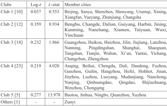
Table 3: Initial convergence club classification of the SPI-S (second-hand house
market): 69 large and medium-sized cities Clubs Log-t t -stat Member cities
Club 1 [10] 0.037 0.553 Beijing, Sanya, Shenzhen, Shenyang, Urumqi, Xining, Xiangfan, Yueyang, Zhanjiang, Changsha
Club 2 [12] 0.359 8.934 Bengbu, Changde, Dalian, Guiyang, Harbin, Jining, Kunming, Nanchang, Xiamen, Taiyuan, Wuxi, Yinchuan
Club 3 [18] 0.232 1.866 Guangzhou, Haikou, Huizhou, Jilin, Jiujiang, Lanzhou, Nanning, Pingdingshan, Shanghai, Shaoguan, Tangshan, Tianjin, Wuhan, Xi’an, Yantai, Yichang, Changchun, Zhengzhou
Club 4 [23] 0.219 4.020 Anqing, Beihai, Chengdu, Dali, Dandong, Fuzhou, Ganzhou, Guilin, Hangzhou, Hefei, Hohhot, Jinan, Jinzhou, Luzhou, Luoyang, Mudanjiang, Nanchong, Nanjing, Qinhuangdao, Qingdao, Shijiazhuang, Wenzhou, Chongqing
Club 5 [5] 0.277 13.978 Baotou, Jinhua, Ningbo, Quanzhou, Xuzhou
Others [1] - - Zunyi
Source: Organized by the authors according to running results of the clustering procedure mentioned above
Note for Table 1~3: (a) t-stat is the convergence test statistic, which is distributed as a simple one-sided t-test with a critical value of -1.65 (see Phillips and Sul, 2007 for more details). (b) Entries in square brackets represent the number of cities in a convergence club. (c) * Denotes the rejection of the convergence null hypothesis at 5% significance level.
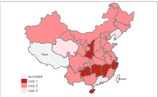
As seen from the results of merged clubs, we could obtain partial evidence that
members in each club are geographically neighboring (see Figure 3), but this
kind of neighboring seems to be quite different from that in conventional Chinese economic regions (East, Central, West and Northeast).
Figure 3: Final house price convergence club classification for the ASHP: 30 regions ExcelPro的图表博客 Tibet Taiwan excluded club 1 club 2 club 3
Source: Organized by the authors according to running results of the clustering procedure mentioned above
Table 4 presents the convergence test results in each of the four regions for all of the three indicators.
Table 4: Convergence test results for ASHP, SPI-N and SPI-S: economic regions Regions the ASHPt -stat for (new-hand house market) t -stat for the SPI-N (second-hand house market)t -stat for the SPI-S
East -24.612 -14.454 -11.228
Central -113.760 -12.610 -659.801
West -24.910 -47.138 -18.994
Northeast -35.794 -12.835 -116.810
Source: Organized by the authors according to running results of convergence test
From the results, we could find little evidence of convergence for each of the
four regions because all of the t-stat values are smaller than -1.65. We even run
the convergence tests for another Chinese economic division on city level (First-tier cities, Second-(First-tier cities, Third-(First-tier cities and Fourth-(First-tier cities and others)13. 13 To conserve on space, we do not report a list of members in each tier of cities and the convergence
However, we still could not find any evidence of convergence within such regions. Thus, we conclude that the conventional definitions of economic regions may not
be appropriate for analyzing house price segregation in China, which is the same
case with the USA found by Kim et al. (2012).
4.3. Dynamic analysis of the convergence
Since the Chinese central government has implemented a series of policies and regulations to control the excessive increase of house prices especially since the
end of 2009, we have chosen all five dates when important housing policies were
issued and repeated the cluster analysis with varying the end of the sample size from 2008:M1 to 2013:M12 to examine the impact of those policies and regulations on China’s housing market.
Figure 4: P-values of the Kruskal-Wallis for the ASHP: 30 regions
Note: (a) This figure reflects the p-values of the Kruskal-Wallis (KW) statistics when they are applied to the results of the cluster analysis for the sample sizes that cover the period 2001:M1-x, with x=2008:M1, …, 2013:M12. (b) All five circles mark the dates when important housing policies were issued. In detail, green circle marks policies aiming to stimulate the housing market, while red circle marks policies to curb the house price. Source: Organized by the authors according to running results of
Wallis test
From the results, firstly we can see a clear alteration of the clustering clubs over time,
because the number of clubs falls when the sample size increases for all of the three indicators: the ASHP (5 clubs in 2008:M1 to 3 clubs in 2013:M12), the SPI-N and
the SPI-S (see Figure 5)14. Then, in order to obtain further statistical evidence of
the change, we have applied the Kruskal-Wallis to test whether those clubs in each
period have been generated by the same general distribution by following Montañés
et al.(2013). Figure 4 shows the evolution of the p-values. It is straightforward to see
that the null hypothesis could be rejected at the time points of 2009:M4, 2010:M9,
2011:M6~M12 and 2013:M7 where all of the p-values are below 5%, which implies that the number and the composition of the clubs have altered at those time points. What is more important is that almost each of the start of those time points is 4 or 5 months after the issue of a certain important housing policy. In sum, we can conclude that important housing policies from the central government can alter China’s housing
market, but significantly only in 4 to 5 months after they are issued.
Figure 5: Comparison of the club numbers between the SPI-N (new house market)
and the SPI-S (second-hand house market) over periods
Note: This figure reflects the numbers of the clustering clubs for the SPI-N and the SPI-S with the sample sizes that cover the period 2005:M7-x, with x=2011:M12, …, 2014:M2.
Source: Organized by the authors according to clustering results
Figure 5 not only presents the evolution of the number of the clustering clubs for
the SPI-N and the SPI-S over periods, but also implies the different behaviors between the new house market and the second-hand house market. It is in over 59% of the periods that the two sub-markets have different numbers of clustering clubs. Even when the two submarkets have the same number of clubs at the same period, they have quite different club members. Table 5 and 6 report some of these results. Therefore, we can conclude that the new house market and the second-hand house market in China do not behave the same over time and tend to gather into different clusters at the end. This could support the way of the central government to make housing policies aiming at different sub-markets of the two15.
15 On February 20, 2013, the Chinese central government required that sellers would be taxed 20%
Table 5: Effect of changing the end of the sample on the cluster analysis for the SPI-N (new house market): 69 large and medium-sized cities
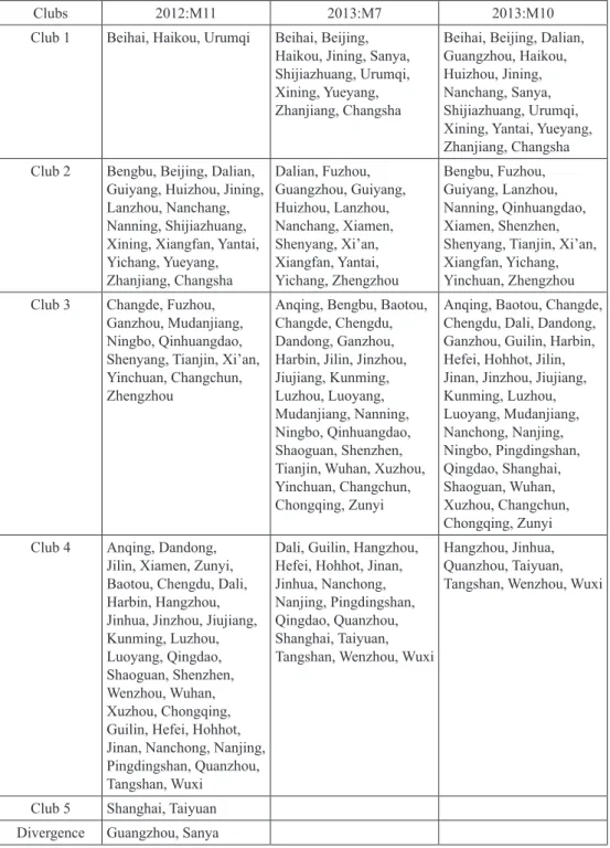
Clubs 2012:M11 2013:M7 2013:M10
Club 1 Beihai, Haikou, Urumqi Beihai, Beijing, Haikou, Jining, Sanya, Shijiazhuang, Urumqi, Xining, Yueyang, Zhanjiang, Changsha
Beihai, Beijing, Dalian, Guangzhou, Haikou, Huizhou, Jining, Nanchang, Sanya, Shijiazhuang, Urumqi, Xining, Yantai, Yueyang, Zhanjiang, Changsha Club 2 Bengbu, Beijing, Dalian,
Guiyang, Huizhou, Jining, Lanzhou, Nanchang, Nanning, Shijiazhuang, Xining, Xiangfan, Yantai, Yichang, Yueyang, Zhanjiang, Changsha Dalian, Fuzhou, Guangzhou, Guiyang, Huizhou, Lanzhou, Nanchang, Xiamen, Shenyang, Xi’an, Xiangfan, Yantai, Yichang, Zhengzhou Bengbu, Fuzhou, Guiyang, Lanzhou, Nanning, Qinhuangdao, Xiamen, Shenzhen, Shenyang, Tianjin, Xi’an, Xiangfan, Yichang, Yinchuan, Zhengzhou Club 3 Changde, Fuzhou,
Ganzhou, Mudanjiang, Ningbo, Qinhuangdao, Shenyang, Tianjin, Xi’an, Yinchuan, Changchun, Zhengzhou
Anqing, Bengbu, Baotou, Changde, Chengdu, Dandong, Ganzhou, Harbin, Jilin, Jinzhou, Jiujiang, Kunming, Luzhou, Luoyang, Mudanjiang, Nanning, Ningbo, Qinhuangdao, Shaoguan, Shenzhen, Tianjin, Wuhan, Xuzhou, Yinchuan, Changchun, Chongqing, Zunyi
Anqing, Baotou, Changde, Chengdu, Dali, Dandong, Ganzhou, Guilin, Harbin, Hefei, Hohhot, Jilin, Jinan, Jinzhou, Jiujiang, Kunming, Luzhou, Luoyang, Mudanjiang, Nanchong, Nanjing, Ningbo, Pingdingshan, Qingdao, Shanghai, Shaoguan, Wuhan, Xuzhou, Changchun, Chongqing, Zunyi Club 4 Anqing, Dandong,
Jilin, Xiamen, Zunyi, Baotou, Chengdu, Dali, Harbin, Hangzhou, Jinhua, Jinzhou, Jiujiang, Kunming, Luzhou, Luoyang, Qingdao, Shaoguan, Shenzhen, Wenzhou, Wuhan, Xuzhou, Chongqing, Guilin, Hefei, Hohhot, Jinan, Nanchong, Nanjing, Pingdingshan, Quanzhou, Tangshan, Wuxi
Dali, Guilin, Hangzhou, Hefei, Hohhot, Jinan, Jinhua, Nanchong, Nanjing, Pingdingshan, Qingdao, Quanzhou, Shanghai, Taiyuan, Tangshan, Wenzhou, Wuxi
Hangzhou, Jinhua, Quanzhou, Taiyuan, Tangshan, Wenzhou, Wuxi
Club 5 Shanghai, Taiyuan Divergence Guangzhou, Sanya
Table 6: Effect of changing the end of the sample on the cluster analysis for the SPI-S (second-hand house market): 69 large and medium-sized cities
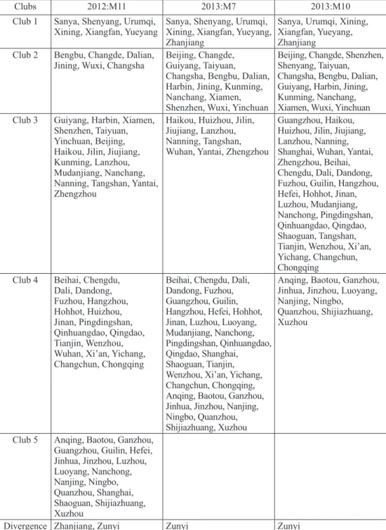
Clubs 2012:M11 2013:M7 2013:M10
Club 1 Sanya, Shenyang, Urumqi,
Xining, Xiangfan, Yueyang Sanya, Shenyang, Urumqi, Xining, Xiangfan, Yueyang, Zhanjiang
Sanya, Urumqi, Xining, Xiangfan, Yueyang, Zhanjiang
Club 2 Bengbu, Changde, Dalian,
Jining, Wuxi, Changsha Beijing, Changde, Guiyang, Taiyuan, Changsha, Bengbu, Dalian, Harbin, Jining, Kunming, Nanchang, Xiamen, Shenzhen, Wuxi, Yinchuan
Beijing, Changde, Shenzhen, Shenyang, Taiyuan, Changsha, Bengbu, Dalian, Guiyang, Harbin, Jining, Kunming, Nanchang, Xiamen, Wuxi, Yinchuan Club 3 Guiyang, Harbin, Xiamen,
Shenzhen, Taiyuan, Yinchuan, Beijing, Haikou, Jilin, Jiujiang, Kunming, Lanzhou, Mudanjiang, Nanchang, Nanning, Tangshan, Yantai, Zhengzhou
Haikou, Huizhou, Jilin, Jiujiang, Lanzhou, Nanning, Tangshan, Wuhan, Yantai, Zhengzhou
Guangzhou, Haikou, Huizhou, Jilin, Jiujiang, Lanzhou, Nanning, Shanghai, Wuhan, Yantai, Zhengzhou, Beihai, Chengdu, Dali, Dandong, Fuzhou, Guilin, Hangzhou, Hefei, Hohhot, Jinan, Luzhou, Mudanjiang, Nanchong, Pingdingshan, Qinhuangdao, Qingdao, Shaoguan, Tangshan, Tianjin, Wenzhou, Xi’an, Yichang, Changchun, Chongqing
Club 4 Beihai, Chengdu, Dali, Dandong, Fuzhou, Hangzhou, Hohhot, Huizhou, Jinan, Pingdingshan, Qinhuangdao, Qingdao, Tianjin, Wenzhou, Wuhan, Xi’an, Yichang, Changchun, Chongqing
Beihai, Chengdu, Dali, Dandong, Fuzhou, Guangzhou, Guilin, Hangzhou, Hefei, Hohhot, Jinan, Luzhou, Luoyang, Mudanjiang, Nanchong, Pingdingshan, Qinhuangdao, Qingdao, Shanghai, Shaoguan, Tianjin, Wenzhou, Xi’an, Yichang, Changchun, Chongqing, Anqing, Baotou, Ganzhou, Jinhua, Jinzhou, Nanjing, Ningbo, Quanzhou, Shijiazhuang, Xuzhou
Anqing, Baotou, Ganzhou, Jinhua, Jinzhou, Luoyang, Nanjing, Ningbo, Quanzhou, Shijiazhuang, Xuzhou
Club 5 Anqing, Baotou, Ganzhou, Guangzhou, Guilin, Hefei, Jinhua, Jinzhou, Luzhou, Luoyang, Nanchong, Nanjing, Ningbo, Quanzhou, Shanghai, Shaoguan, Shijiazhuang, Xuzhou
Divergence Zhanjiang, Zunyi Zunyi Zunyi
4.4. Exploring the driving forces of the convergence
In this part, we select 7 indicators to build a panel data model, namely, economic
fluctuations, land supply, urban residents’ income, credit scale of real estate
development, urban population, city size and house price expectation. Since the data set used in this part is not sampling data but overall data from 30 regions,
fixed effects panel data model has been chosen. In addition, in order to eliminate
heteroscedasticity, we build a semi-logarithmic linear model as follows, where the
coefficients in the model show the elasticity between independent variables and
dependent variable. 0 1 2 3 4 5 6 7 ( ) ( ) ( ) ( ) ( ) ( ) ( (-1)) it it it it it it it it it
ln HP ln ICOME GDPZ ln LAND ln POP
ln LOAN ln CITY ln HP
β β β β β
β β β ε
= + + + +
+ + + + (8)
Where i is cross-sectional index, and t is time-series index. HPit is the house price in region i and time t, ICOMEit is urban residents’ income in region i and time t,
GDPZit reflects economic fluctuation level in region i and time t, LANDit is the land supply in region i and time t, POPit is the urban population of region i in time t,
LOANit is the credit scale in region i and time t, CITYit reflects city size of region i in time t, HPit(-1) is the house price in region i and time t-1, which reflects the house price expectation. β0 is the constant, and β0 ~β7 are the coefficients to be estimated,
εit is the error term.
Stepwise regression is used to select the best model with the highest adjusted R2
and all dependent variables passing t-test. Considering that the historical house
price (reflecting the house price expectation) is the most significant factor affecting
regional house price, and the urban residents’ income is the most important and
the most fundamental factor influencing the effective demand of real estate market,
we add other explanatory variables one by one into the model on the basis of one-lagged house price and per capita disposable income of urban residents.
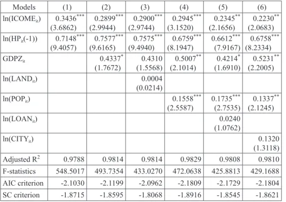
Table 7:The regression results for club 1 Models (1) (2) (3) (4) (5) (6) ln(ICOMEit) 0.3436*** (3.6862) 0.2899 *** (2.9944) 0.2900 *** (2.9744) 0.2945 *** (3.1520) 0.2345 ** (2.1656) 0.2230 ** (2.0683) ln(HPit(-1)) 0.7148*** (9.4057) 0.7577 *** (9.6165) 0.7575 *** (9.4940) 0.6759 *** (8.1947) 0.6612 *** (7.9167) 0.6758 *** (8.2334) GDPZit 0.4337* (1.7672) (1.5568)0.4310 0.5007 ** (2.1014) 0.4214 * (1.6910) 0.5231 ** (2.2005) ln(LANDit) 0.0004 (0.0214) ln(POPit) 0.1558*** (2.5587) 0.1735 *** (2.7535) 0.1337 ** (2.1245) ln(LOANit) 0.0240 (1.0762) ln(CITYit) 0.1320 (1.3118) Adjusted R2 0.9788 0.9814 0.9814 0.9829 0.9808 0.9810 F-statistics 548.5017 493.7354 433.0270 472.0638 425.8813 429.1688 AIC criterion -2.1030 -2.1199 -2.0962 -2.1809 -2.1729 -2.1804 SC criterion -1.8715 -1.8595 -1.8068 -1.8916 -1.8545 -1.8621
Note: (a) t-test values are shown in brackets. (b)***, ** and* each means significance level of 1%,
5% and 10%.
Source: Organized by the authors according to regression results
As model (4) in Table 7 shows that urban residents’ income, house price
expectation, economic fluctuation level and urban population could effectively
explain regional house prices in club 1. Through further theoretical analysis, it’s believed that urban residents’ income and urban population would directly impact the supply and demand of regional real estate market, while economic growth and house price expectation would indirectly affect the house price through urban
residents’ income, asset prices, etc. The empirical analysis above does not find any significant evidence for the effects of land supply, credit scale of real estate
development and city size on regional house price for club 1.
The same method used has been applied to analyze the data of club 2 and club 3. The result of factor analysis with stepwise regression is shown in Table 8.
According to the estimated coefficients, the effect of house price expectation on the real estate market is significant and is similar among all the three club area. The influences of urban residents’ income and economic fluctuation on real estate market are significant in club 1 and 2. Specifically, the effect of economic fluctuation is greater in club 1 than club 2. Also, land supply is preferred to have
an observable impact in club 2, and urban population has significant and similar
impact on real estate market in club 1 and 3. In addition, the effect of credit scale of real estate development is evident in club 2 and 3, and is more obvious in club 3 than that in club 2.
Table 8: Comparisons between regression results of three club
Clubs ln(ICOMEit) ln(HPit(-1)) GDPZit ln(LANDit) ln(POPit) ln(LOANit) ln(CITYit)
club 1 0.2945 0.6759 0.5007 - 0.1558 -
-club 2 0.2810 0.6220 0.2913 -0.0340 - 0.0493
-club 3 - 0.5801 - - 0.1326 0.1030
-Source: Organized by the authors according to regression results
Based on the above analysis, it can be found that the driving forces of the convergence differ among three clubs, which further demonstrates the complexity of housing market in China. Thus, the implementation of housing policies in the three clubs should be differentiated accordingly.
5. Results and discussion
The results of convergence tests show little evidence of overall convergence across regions in China’s housing market, and provide evidence for the existence of some degree of segmentation in China’s housing market. The obtained clubs are quite different from that in conventional Chinese economic regions (East, Central, West and Northeast). And it’s found little evidence of convergence for each of the four
regions and Chinese economic division on city level (First-tier cities, Second-tier cities, Third-tier cities and Fourth-tier cities and others), which indicates that the conventional definitions of economic regions may not be appropriate for analyzing
house price segregation in China.
Furthermore, the dynamics of the convergence is also analyzed, which leads us
to conclude that the housing market in China has evidently altered because the clustering results differ depending on when the sample ends. And we have found
that important housing policies from Chinese central government can significantly alter the housing market but with a time lag of 4 to 5 months. Besides, we also find
that do not behave the same over time and tend to gather into different clusters at the end by comparing the clustering results of the two sub-markets.
Also this research paper finds evidences that multiple factors together have been the
driving forces for the regional house price convergence in China. And the driving forces differ among three clubs. Thus, the implementation of housing policies in the three clubs should be differentiated accordingly.
6. Conclusions
On the basis of the obtained results, the hypothesis that there is segmentation across
regions in China’s housing market is confirmed. Heterogeneous convergence exists
in China’s regional house prices and there is not a single common convergence factor in China’s housing market, which indicates the complexity of regional house prices in China. The obtained results of this research provide the new fact for the economic science respectively economic literature. However this research has also got the certain
limitations. For instance, the dynamic of China’s housing price and its driving forces
are pretty complicated, which differ apparently among different regions, especially at city level. In this research, we analyzes the convergence of regional house prices at provincial level. The future research have to be directed toward the convergence of housing price at city level in China. The obtained results can also provide implications for the implementation of differentiated housing policies.in China: 1) it’s important to effective manage housing price expectation for all the regions. 2) Housing policies
should be implemented with different focus among the regions. For instance, the
reasonable plan of urban land supply is crucial for housing market in club 2. 3) The way of the central government to make housing policies aiming at different sub-markets of the new house market and the second-hand house market.
References
Canarella, G., Miller, S., Pollard, S. (2012) “Unit Roots and Structural Change: An
Application to Us House Price Indices”,Urban Studies, Vol. 49, No. 4, pp.757– 776, doi: 10.1177/0042098011404935.
Catmull, E., Rom, R. (1974) “A Class of Local Interpolating Splines”. Computer
Aided Geometric Design, Vol. 74, pp. 317–326, doi:
10.1016/B978-0-12-079050-0.50020-5.
Chen F., Wang L.J. (2000) “Regional differences of the marketization of China’s
real estate market and the development strategy”. The Theory and Practice
of Finance and Economics Vol. 21, No. 3, pp. 104–107. (in Chinese), doi:
10.3969/j.issn.1003-7217.2000.03.040.
Chen Z.X., Huang Z. (2010) “Research on the interaction of real estate prices in the
Pearl River Delta - Taking Guangzhou, Shenzhen, Dongguan as an example”.
South China Finance, No. 4, pp. 82–86. in Chinese), doi:
10.3969/j.issn.1007-9041.2010.04.021.
Clark S. P., Coggin T.D. (2009) “Trends, cycles and convergence in US regional
house prices”, The Journal of Real Estate Finance and Economics, Vol. 39, No. 3, pp. 264–283, doi: 10.1007/s11146-009-9183-1.
Cook, S. (2003) “The Convergence of Regional House Prices in the UK”. Urban
Cooper C, Orford S, Webster C., et al. (2013) “Exploring the Ripple Effect and Spatial
Volatility in House Prices in England and Wales, Regressing Interaction Domain Cross-Correlations Against Reactive Statistics”. Environment and Planning B, Planning and Design, Vol. 40, No. 5, pp. 763–782, doi: 10.1068/b37062.
Downes, T.A., Zabel, J.E. (2002) “The Impact of School Characteristics on House
Prices: Chicago 1987–1991”. Journal of Urban Economics, Vol. 52, No. 1, pp. 1–25, doi: 10.1016/s0094-1190(02)00010-4.
Gabriel, S.A., Rosenthal, S.S. (1989) “Household Location and Race: Estimates of
A Multinomial Logit Model”. Review of Economics and Statistics, Vol. 71, No. 2, pp.240–249, doi: 10.2307/1926969.
Gallin, J. (2006) “The Long-Run Relationship between House Prices and Income:
Evidence from Local Housing Markets”. Real Estate Economics, Vol. 34, No. 3, pp. 417–438. doi: 10.1111/j.1540-6229.2006.00172.x.
Ghysels, E., Perron, P. (1993) “The Effect of Seasonal Adjustment Filters on Tests
for A Unit Root”. Journal of Econometrics, Vol. 55, No. 1, pp. 57-98, doi: 10.1016/0304-4076(93)90004-O.
Gupta R., Miller S.M. (2012) “Ripple effects and forecasting home prices in Los
Angeles, Las Vegas and Phoenix”. The Annals of Regional Science, Vol. 48, No. 3, pp. 763–782, doi: 10.1007/s00168-010-0416-2.
Haurin, D.R., Brasington, D. (1996). “School Quality and Real House Prices:
Inter-and Intra-Metropolitan Effects”. Journal of Housing Economics, Vol. 5, No. 4, pp. 351–368. doi: 10.1006/jhec.1996.0018.
Herrerias, M.J., Ordoñez, J. (2012) “New Evidence on the Role of Regional
Clusters and Convergence in China (1952–2008)”. China Economic Review, Vol.23, No. 4, pp. 1120–1133, doi: 10.1016/j.chieco.2012.08.001.
Hodrick, R., Prescott, E. (1997) “Post-war US Business Cycles: A Descriptive
Empirical Investigation”. Journal of Money Credit and Banking, Vol. 29, No. 1, pp. 1–16, doi: 10.2307/2953682.
Hwang, M., Quigley, J. M. (2006) “Economic Fundamentals in Local Housing
Markets: Evidence from US Metropolitan Regions”. Journal of Regional
Science, Vol. 46, No. 3, pp. 425–453, doi: 10.1111/j.1467-9787.2006.00480.x.
Kiel, K.A., Zabel, J.E. (2008) “Location, Location, Location: The 3L Approach to
House Price Determination”. Journal of Housing Economics, Vol. 17, No. 2, pp. 175–190, doi: 10.1016/j.jhe.2007.12.002.
Kim, Y.S., Rous, J.J. (2012) “House Price Convergence: Evidence from US State
and Metropolitan Area Panels”. Journal of Housing Economies, Vol. 21, No. 2, pp. 159–186, doi: 10.1016/j.jhe.2012.01.002.
MacDonald, R., Taylor, M.P. (1993) “Regional House Prices in Britain:
Long-Run Relationships and Short-Long-Run Dynamics”. Scottish Journal of Political
Meen, G. (2002) “The Time-Series Behavior of House Prices: A Transatlantic
Divide?” Journal of Housing Economics, Vol. 11, No. 1, pp. 1–23. doi: 10.1006/ jhec.2001.0307.
Mikhed, V., Zemčík, P. (2009) “Do House Prices Reflect Fundamentals? Aggregate
and Panel Data Evidence” Journal of Housing Economics, Vol. 18, No. 2, pp. 140–149, doi: 10.1016/j.jhe.2009.03.001.
Miles, W. (2015) “Regional House Price Segmentation and Convergence in the US:
A New Approach”, Journal of Real Estate Finance and Economics, Vol. 50, No. 1, pp. 1–16, doi: 10.1007/s11146-013-9451-y.
Montañés, A., Olmos, L. (2013). “Convergence in US House Prices” Economics
Letters, Vol. 121, No. 2, pp. 152–155, doi: 10.1016/j.econlet.2013.07.021.
Ng, S., & Perron, P. (2001) “Lag Length Selection and the Construction of Unit
Root Test with Good Size and Power” Econometrica, Vol. 69, No. 6, pp. 1519–1554; doi: 10.1111/1468-0262.00256.
Phillips, P.C., Sul, D. (2007) “Transition Modelling and Econometric Convergence
Tests”. Econometrica, Vol. 75, No. 6, pp. 1771–1855, doi: 10.1111/j.1468-0262.2007.00811.x.
Phillips, P.C., Sul, D. (2009) “Economic Transition and Growth”. Journal of
Applied Econometrics, Vol. 24, No. 7, pp. 1153–1185, doi: 10.1002/jae.1080.
Wei Z.Y., Yang Z.Z. (2007) “Dynamic Consistency Research on Change of Housing Price in Yangtze River Delta”, Journal of Nanjing Normal University (Social Science Edition), No. 3, pp. 43–48, in Chinese), doi: 10.3969/j.issn.1001-4608-B.2007.03.007.
Zhang S.L., Zhang H.B., Wang Q. (2011) “An empirical study on house price
transmission mechanism among Huanbohai region”, Journal of Hebei
University (Philosophy and Social Science), Vol. 36, No. 3, pp. 85–90, in Chinese), doi: 10.3969/j.issn.1000-6378.2011.03.016.
Zhang, F., Morley, B. (2014) “The Convergence of Regional House Prices in
China”. Applied Economics Letters, Vol. 21, No. 3, pp. 205–208, in Chinese), doi: 10.1080/13504851.2013.848021.
Heterogena konvergencija i kompleksnost regionalnih cijena kuća u Kini
1Rui Lin2, Xin Zhang3, Xiuting Li4, Jichang Dong5
Sažetak
Svrha ovog istraživanja je analizirati konvergenciju i kompleksnost regionalnih cijena kuća i u Kini. U tu svrhu koristi se model nelinearnih vremenski promjenjivih faktora. Dobiveni rezultati potvrđuju postojanje određenog stupnja segmentacije kineskog tržišta nekretnina. Daljnjom dinamičkom analizom konvergencije utvrđeno je da kineska središnja vlast svojom važnom stambenom politikom može značajno utjecati na promjenu tržišta nekretnina, ali s vremenskim odmakom od 4 do 5 mjeseci, i da su sasvim različita ponašanja između stambenog tržišta novogradnja i tržišta starijih stambenih objekata u Kini što dokazuje složenost tržišta nekretnina u Kini. Višestruki čimbenici zajedno su pokretači konvergencije cijena regionalnih stambenih objekata, a pokretačka snaga razlikuje se u tri kluba. Temeljni zaključak iz provedenih istraživanja je da konvencionalne definicije ekonomskih regija nisu prikladne za analizu segregacije cijena stambenih objekata u Kini. U Kini postoji heterogena konvergencija regionalnih cijena kuća, što ukazuje na kompleksnost regionalnih cijena nekretnina. Stambena politika treba se provoditi različito u različitim regijama. Način na koji središnja vlada treba provoditi stambenu politiku je da bude usmjerena na različita pod-tržišta stambenih novogradnja i tržišta korištenih stambenih objekata.
Ključne riječi: konvergencija, cijena kuća, Kina, politika, kompleksnost JEL klasifikacija:E30, P25, R11
1 Ovaj rad nastao je uz potporu Nacionalne prirodoslovne zaklade Kine (The National Natural Science Foundation of China; Grant br. 71173213; Grant br. 71203217; 71403260) i Kineske postdoktorske zaklade za znanost (The China Postdoctoral Science Foundation, Grant br. 2013M540129).
2 Doktor ekonomskih znanosti, School of Economics and Management, University of Chinese Academy of Sciences, Beijing 100190, Kina. Department of Sociology, University of Chicago, 5801 S Ellis Ave, Chicago, IL 60637, SAD. Znanstveni interes: ekonomika nekretnina. Tel: +86 15201305859. E-mail: linrui0704@163.com. Web stranica: http://www.mscas.ac.cn/.
3 Doktor ekonomskih znanosti, School of Economics and Management, University of Chinese Academy of Sciences, Beijing 100190, Kina. Znanstveni interes: ekonomika nekretnina. Tel.: +86 1 8810 404 354. E-mail: zhangxin2970@163.com. Web stranica: http://www.mscas.ac.cn/. 4 Docent, School of Economics and Management, University of Chinese Academy of Sciences, Beijing 100190, Kina. Znanstveni interes: ekonomika nekretnina, bihevioralne financije. Tel.: +86 1 3811 580 462. E-mail: lixiuting@ucas.ac.cn. Web stranica: http://www.mscas.ac.cn/ Teachers/Professor/243.shtml. (kontakt osoba).
5 Redoviti profesor, School of Economics and Management, University of Chinese Academy of Sciences, Beijing 100190, Kina. Znanstveni interes: ekonomika nekretnina, financijski inženjering. Tel.: +86 1 3521 211 972. E-mail: jcdonglc@ucas.ac.cn. Web stranica: http:// www.mscas.ac.cn/Teachers/Professor/201.shtml.