www.elsevier.com / locate / econbase
German monetary unification and the stability of the German
M3 money demand function
a ,
*
bMohsen Bahmani-Oskooee
, Martin T. Bohl
a
Department of Economics, The University of Wisconsin-Milwaukee, Milwaukee, WI 53201, USA
b
Department of Economics, Justus-Liebig University of Giessen, Licher Street 74, 35394 Giessen, Germany Received 21 December 1998; accepted 12 May 1999
Abstract
This paper employs quarterly data from the whole of Germany to test the stability of M3 demand for money. The methodology is based on an application of the CUSUM and CUSUMSQ in the context of error-correction modeling and cointegration. The results reveal some instability in M3 money demand function. 2000 Elsevier Science S.A. All rights reserved.
Keywords: CUSUM; CUSUMSQ; Cointegration; M3; Germany
JEL classification: E41
1. Introduction
The German Monetary Unification (GMU) in 1990 has resulted in a lively debate over the existence of a stable whole-German money demand function. If unification causes instability in the money demand function, then Deutsche Bundesbank would lose one of the fundamental preconditions for an effective implementation of its anti-inflationary monetary policy. Thus, it is important to establish the stability of the whole-German money demand function.
Few studies have investigated the stability of German money demand function after unification. von Hagen (1993) investigated stability of M1 and M3 velocity equation using quarterly whole-German data over 1965I–1991IV period. By employing general-to-specific specification methodology of Hendry (1979) and Hendry et al. (1984) and by relying on out of sample prediction tests for structural stability, von Hagen (1993) finds a stable M1 velocity, but an unstable M3 velocity. Falk and Funke (1995) use quarterly data over 1977IV–1992IV period and the error-correction (EC)-based approach
*Corresponding author. Fax: 11-414-229-3860.
E-mail address: [email protected] (M. Bahmani-Oskooee)
proposed by Kremers et al. (1992) to investigate the stability of only M1 money demand function. They reject the null of no cointegration and find some evidence of instability by plotting the recursive long-run income and interest elasticity. Hansen and Kim (1995) investigate the stability of M1 using data over 1960I–1992IV period and M3 using data over the 1974I–1992IV period. They find a cointegrating relation among the variables of M3 using Quintos and Phillips (1993) LM test, but no cointegration using Hansen (1992) LMP test. However, conventional sample split tests for structural break and Hansen (1992) SupF tests indicate instability in 1990 due to unification.
¨
Issing and Todter (1995) investigated the stability of only M3 money demand function using quarterly data over the 1975I–1993II period. Their empirical findings reveal the existence of a cointegrating relation, and the Chow forecast test shows no instability of M3 money demand function due to unification. The same result is confirmed by Clostermann et al. (1997) when they apply the Johansen (1988) cointegration technique and the Hansen (1992) SupF, MeanF and LMP tests. The stability is confirmed by showing minor fluctuation of the eigenvalues without any statistical test and elaboration.
In this paper we try to investigate the stability of the M3 money demand function for the whole of Germany by incorporating the short-run dynamics in testing for the long-run income and interest elasticities. Section 2 introduces the testing procedure and empirical results. Section 3 concludes. Finally, data definition and sources are cited in Appendix A.
2. The method and the results
Following the literature, we assume that income and interest rate are the main determinants of the demand for M3. Thus, the following formulation in log linear form is adopted:
ln M3 5a1b ln Y 1c ln i1e (1)
t t t
where M3 is the real monetary aggregate (M3); Y is the real income with expected positive elasticity and i is a measure of opportunity cost of holding money, i.e., long-run interest rate with expected negative elasticity.
We first try to estimate Eq. (1) for the whole of Germany using seasonally adjusted quarterly data over the 1969I–1995IV period. We begin with 1969 because seasonally adjusted M3 begins with that date, and 1995IV was the last date for which seasonally adjusted data was available. Since the estimation procedure is based on the cointegration technique of Johansen and Juselius (1990), we first determine the degree of integration of each variable in (1). To this end, we employ the Kwiatkowski et al. (1992) test, known as the KPSS test. The KPSS test is formulated in Bahmani-Oskooee (1998) and needs no repeat here. The results are reported in Table 1.
Table 1
The KPSS test results (Panel A) the KPSS statistics for null of level stationary (the 5 and 10% critical values are 0.463 and 0.347 respectively) and (Panel B) the KPSS statistics for null of trend stationary (the 5 and 10% critical values are 0.146 and 0.119, respectively)
Lag truncation parameter
Variable 0 1 2 3 4 5 6 7 8
Panel A:
ln M3 10.52 5.337 3.598 2.727 2.204 1.856 1.608 1.422 1.279
ln Y 10.15 5.169 3.493 2.653 2.148 1.812 1.572 1.392 1.253
ln i 1.340 0.696 0.483 0.378 0.316 0.277 0.250 0.231 0.217
Panel B:
ln M3 0.903 0.477 0.333 0.261 0.218 0.189 0.169 0.154 0.143
ln Y 1.327 0.689 0.470 0.361 0.295 0.252 0.222 0.200 0.183
ln i 0.249 0.130 0.091 0.071 0.060 0.053 0.048 0.045 0.042
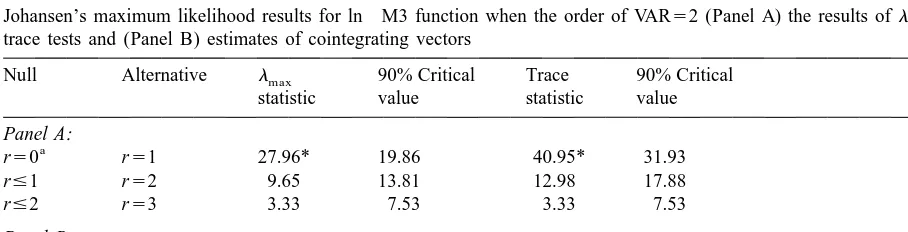
We are now in a position to apply Johansen and Juselius (1990) cointegration analysis which is based on the maximum-likelihood estimation technique. They introduce two test statistics known as
lmax and trace to identify number of cointegrating vectors. These two statistics are reported in Panel A
of Table 2. Note that in selecting the order of VAR, we employed AIC criterion which selected two lags.
From Panel A of Table 2 it is clear that the null of no cointegration is rejected by both statistics because either statistic is larger than the critical value (indicated by *). However, the null of at most one vector cannot be rejected in favor of r52. Thus, there is only one cointegrating vector. The
estimate of this vector normalized on ln M3 is reported in Panel B of Table 2.
We now turn to the stability of the long-run coefficient estimates by taking into consideration the short-run dynamics. To this end, following Pesaran and Pesaran (1997) we form an EC term using the long-run coefficient estimates from panel B of Table 2 and employ its lagged value in the following EC model:
Table 2
Johansen’s maximum likelihood results for ln M3 function when the order of VAR52 (Panel A) the results ofl and
max
trace tests and (Panel B) estimates of cointegrating vectors
Null Alternative l 90% Critical Trace 90% Critical
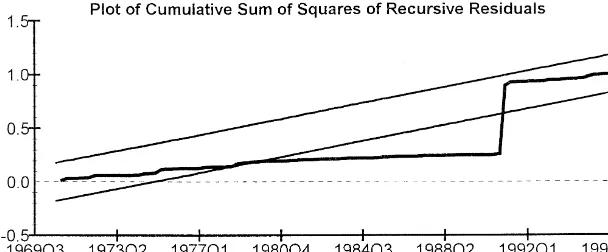
Fig. 1. Plots of CUSUMSQ and CUSUM statistics.
n n n
Dln M3 5a1
O
b Dln M3 1O
c Dln Y 1O
d Di 1lEC 1e (2)t j t2j j t2j j t2j t21 t
j51 j51 j51
Pesaran and Pesaran (1997) then suggest employing CUSUM or CUSUMSQ tests proposed by Brown et al. (1975). The CUSUM and CUSUMSQ statistics are updated recursively and are plotted against the break points. If the plot of CUSUM or CUSUMSQ stay within 5% significance level (portrayed by two straight lines whose equations are given in Brown et al., 1975, Section 2.3), then the coefficient estimates are said to be stable. A graphical presentation of the tests are provided in Fig. 1.
It is clear from Fig. 1 that at least the plots of CUSUMSQ statistic crosses the critical bounds,
1
indicating that short-run and long-run elasticities are unstable.
1
3. Summary and conclusion
The stability of the money demand function in any country is of great importance for a successful monetary policy. The unification of the West and East German states in 1990 has been considered as a new factor that may result is instability of the money demand in unified Germany. There are few studies that have considered stability of German money demand after unification, with mixed results. In this paper we investigated the stability of German money demand. The paper differs from previous studies in that it incorporates the short-run dynamics in testing for the stability of long-run M3 money demand function. This is done by testing for the stability of all estimated coefficients in an EC model. The results obtained from applying the CUSUMSQ test revealed instability in the whole German M3 money demand function.
Appendix A
A.1. Data definitions and sources
All data are quarterly over the period 1969I–1995IV and obtained from the following sources:
(a) main Economic Indicators of OECD; (b) International Financial Statistics of IMF;
(c) Saisonbereinigte Wirtschaftszahlen of the Deutsche Bundesbank; (d) Kapitalmarktstatistik of the Bundesbank;
A.2. Variables
M15real M1. Seasonally adjusted nominal M1 figures from source (a) are deflated by seasonally
adjusted GDP deflator (19915100) from source (c) to obtain this measure.
M25real M2. Seasonally adjusted nominal M2 figures from source (a) are deflated by seasonally
adjusted GDP deflator (19915100) from source (c).
M35real M3. Seasonally adjusted nominal M3 figures from source (b) are updated from source (c).
They are then deflated by seasonally adjusted GDP deflator (19915100) from source (c).
Y5real GDP. Seasonally adjusted real GDP (in 1991 prices) comes from source (c). i5long-term
government bond yield obtained from source (d).
References
Bahmani-Oskooee, M., 1998. Do exchange rates follow a random walk process in Middle Eastern Countries? Economic Letters 58, 339–344.
¨ ¨
Falk, M., Funke, N., 1995. The stability of money demand in Germany and in the EMS: impact of German Unification. Weltwirtschaftliches Archiv 131, 470–488.
Hansen, B.E., 1992. Tests for parameter instability in regressions with I(1) processes. Journal of Business and Economic Statistics 10, 312–335.
Hansen, G., Kim, J.R., 1995. The stability of German money demand: tests of the cointegration relation. Weltwirtschaftliches Archiv 131, 286–301.
Hendry, D.F., 1979. Predictive failure and Econometric Modelling in macroeconomics: the transactions demand for money, in modelling the economy. In: Ormerod, P. (Ed.), Heinemann, London.
Hendry, D.F., Pagan, A.R., Sargan, J.D., 1984. In: Grilichs, Z., Intriligator, M.D. (Eds.), Dynamic Specification in Handbook of Econometrics, North Holland, Amsterdam.
¨
Issing, O., Todter, K.H., 1995. Geldmenge und Preise im vereinten Deutschland, in Neuere Entwicklungen in der
¨ ¨
Geldtheorie und Wahrungspolitik. In: Duwendag, D. (Ed.), Schriften des Vereins fur Socialpolitik 235, Duncker und Humbolt, Berlin.
Johansen, S., Juselius, K., 1990. Maximum likelihood estimation and inference on cointegration — with applications to the demand for money. Oxford Bulletin of Economics and Statistics 52, 169–210.
Kremers, J.J.M., Ericsson, N.R., Dolado, J.J., 1992. The power of cointegration tests. Oxford Bulletin of Economics and Statistics 54, 777–805.
Kwiatkowski, D., Phillips, P.C.B., Schmidt, P., Shin, Y., 1992. Testing the null hypothesis of stationarity against the alternative of a unit root. Journal of Econometrics 54, 159–178.
Pesaran, H.M., Pesaran, B., 1997. In: Microfit 4.0, An Interactive Econometric Analysis, Camfit Data, UK.
Quintos, C.E., Phillips, P.C.B., 1993. Parameter constancy in cointegrating regressions. Empirical Economics 18, 675–706. von Hagen, J., 1993. Monetary Union, money demand, and money supply: a review of the German Monetary Union.