RANDOM FORESTS-BASED FEATURE SELECTION
FOR LAND-USE CLASSIFICATION USING LIDAR DATA AND ORTHOIMAGERY
Haiyan Guana, Jun Yub, Jonathan Lia,b*, Lun Luoc
aGeoSTARS Lab, Department of Geography and Environmental Management, University of Waterloo, 200 University
Ave. West, Waterloo, ON, Canada N2L 3G1
bGeoSTARS Group, School of Information Science and Engineering, Xiamen University, 422 Siming Road South,
Xiamen, Fujian, China 361005
cChina Transport Telecommunication & information Center, Beijing, China
KEY WORDS: Lidar, imagery, Random Forests, Classification, Feature selection
ABSTRACT:
The development of lidar system, especially incorporated with high-resolution camera components, has shown great potential for urban classification. However, how to automatically select the best features for land-use classification is challenging. Random Forests, a newly developed machine learning algorithm, is receiving considerable attention in the field of image classification and pattern recognition. Especially, it can provide the measure of variable importance. Thus, in this study the performance of the Random Forests-based feature selection for urban areas was explored. First, we extract features from lidar data, including height-based, intensity-based GLCM measures; other spectral features can be obtained from imagery, such as Red, Blue and Green three bands, and GLCM-based measures. Finally, Random Forests is used to automatically select the optimal and uncorrelated features for land-use classification. 0.5-meter resolution lidar data and aerial imagery are land-used to assess the feature selection performance of Random Forests in the study area located in Mannheim, Germany. The results clearly demonstrate that the use of Random Forests-based feature selection can improve the classification performance by the selected features.
1. INTRODUCTION
Urban land cover classification has always been critical due to its ability to link many elements of human and physical environments. Timely, accurate, and detailed knowledge of the urban land cover information derived from remote sensing data is increasingly required among a wide variety of communities. This surge of interest has been predominately driven by the recent innovations in data, technologies, and theories in urban remote sensing. During the past decades, increasing advances in lidar technologies provide high-accuracy and point-density 3-dimensional point clouds for land-use classification in combination with imagery. As lidar data is unstructured, irregular 3-D points and short of spectral information, classification confusion is often generated between man-made and natural objects. On the other hand, it is difficult to directly obtain land-use information only from remotely sensed data, owing to the complexity of landscapes, spectrally identical objects, as well as abundance of spatial and spectral information. Therefore, integrating lidar point clouds with imagery is being a preferred means for land-use classification.
Although a plethora of features that can be extracted from both lidar point clouds and optical imagery, there is no rule or model for how to automatically and objectively select proper features for the desired classification results. Majority of existing research works are focusing on the development of classification methods, few attentions are paid on the feature selection using lidar data and imagery. The subjective selection of classification features causes the classification results unstable. To this end, Random Forests-based feature selection is proposed in this study.
___________
*junli@uwaterloo.ca, phone1 519-888-4567, ext. 34504
Random Forests, one of ensemble classification family that are trained and their results combined through a voting process, can be considered as an improved version of bagging, a widely used ensemble classifier (Breiman, 1996). It is well known that Random Forests are characterised by notably computational efficiency. In the field of remote sensing, Random Forests has been achieved a promising classification accuracy for hyper-spectral (Wang et al., 2009), multihyper-spectral (Stumpf and Kerle, 2011), and multisource data (Gislason et al., 2006). Due to classification complexity of multisource data, commonly used parametrical classification methods are impropriate. Random Forests, as nonparametric classification algorithm, should be of great interest for multisource data by providing an estimate of individual variable importance index. Moreover, several studies have shown the advantages of Random Forests in land cover classification; the results indicate that the selected features agree the existing physiological knowledge. However, few is focus on urban areas by fusion of lidar data and aerial images. To this end, RF is applied to feature selection in this study.
2. METHOD
2.1 Basic principle of Random Forests
The Random Forests classifier developed by Breiman (2001) is
a combination of decision trees
1, T
k k=
DT x , where x is an
input vector, and k denotes a random vector which is sampled independently but with the same distribution as the past
1, , -1
k . T bootstrap samples are first drawn from the
training data, and then an no pruned classification and regression tree (CART) is grew from each bootstrap sample β where only one of M randomly selected features is chosen for the split at each node of CART. The chosen feature is the one that minimizes the Gini impurity which can be written as (Breiman et al., 1984):
Gini β
f Ci,β β f Cj,β β(1)
where f C
i,β β
is the probability that the randomly selectedpixel belongs to class Ci. Finally, the output of the classifier is determined by a majority vote of all individually trained trees.
There are two parameters: the number of variables (M) in the random subset at each node and the number of trees (T) in the forest. The selection of parameter M has influence on the final error rate. If M is increased, both the correlation between the trees and the strength (classification accuracy) of individual tree in the forest are increased. The error rate is proportional to the correlation, but inverse proportional to the strength (Joelsson et al., 2008). Usually, M is set to the square root of number of features (Gislason et al., 2006). Because Random Forests is fast and not overfit, the number of trees T can be as many as possible. However, due to the memory limit of the machine, T is usually several hundred (Horning, 2010), here is set to 100. The Random Forests also provides two additional measures: the variable importance and internal structure. Variable importance measures the importance of the predictor variables (features). To estimate a feature importance, the OOB samples are first run through the trees and count the votes for the correct classification. Then, the prediction accuracy is repeatedly obtained after randomly permuting all the values of this feature while all the other features stay the same. The importance score is the decrease of the correct class votes after the variable permutation, averaged over all the trees. The intuition is that a random variable permutation can simulates the absence of that variable from the forest (Guo et al., 2011). Thus the higher an average accuracy decrease is, the more important that feature is.
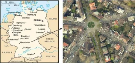
Figure 1. Study area of Mannheim, Germany
2.2 Study Area and Datasets
Laser scanning data covering Mannheim, Germany, were acquired in 2004 by a Falcon II sensor- a Fiber based system concept, TopoSys® GmbH. The airplane flew at an average height of 1,200 m above the mean sea level, with a camera on board for the 0.5m-resolution aerial photographs with RGB bands. The average point density and point spacing within the test site is about 4 points/m2 and 0.5 m, respectively. The lidar dataset records both range (first- and last- returns) and intensity information of the laser pulse. In this research Lidar data is considered in 2D geometry with optical image data. The experimental area is a typical urban region that contains variously sized buildings with different orientations, as well as trees and grass interspersed among buildings. Meanwhile, the study area and its vicinity are relative flat, with elevations ranging from approximately 89.83 m to 159.71 m.
2.3 Training sample and reference data
The training samples are chosen using the photo-interpretation method in the commercial software ENVI®. Table 1 lists the number of training samples. As a proportion of the full image to be analysed the number of training samples would represent less than 1% to 5%. For accuracy assessment, an adequate number of testing data is required per class of interest. Congalton and Green (2009) pointed out that it is necessary to have sufficient testing data for building a valid statistically error matrix to represent classification accuracy. Thus, the sample size N was determined by Equation (2) for the binomial probability theory:
Where p is the expected percent accuracy, E is the allowable error, and Z = 1.96 from the standard normal deviant for the 95% two-sided confidence level. An expected accuracy of 95% was selected because the land-use classification system specifies that each class category should be mapped to at least 85% accuracy, and then the allowable error of 5% is chosen. For this study area, the sample size (N) of 996 meets the demand of Congalton and Green’s (2009) rule-of-thumb of a minimum of 50 samples per class.
Categories Training samples Test data
ROI Pixels ROI Pixels
Buildings 103 927 50 569
High vegetation 36 524 26 421
Ground 60 934 44 685
Grass 12 172 10 98
Table 1. The training samples and test data.
2.4 Features
Aerial Imagery-based (Figure 2(a)):
Three bands (R, G, B): To remove noises in the RGB image, convolution operation must be operated. In this paper, we use median convolution, a technique aiming at reducing image noise without removing significant parts of the image content, typically edges, lines or other details that are important for the interpretation of the image (Perona and Malik, 1990). After mean convolution, bands red (R), green (G) and blue (B) are used as three individual spectral features.
Grey-level Co-occurrence Matrix (GLCM); GLCM proposed by Julesz (1962) can be used to calculate several statistical measures, such as contrast (Cont.), dissimilarity (Diss.), homogeneity (Homo.), entropy (Ent.), mean (Mean), variance (Var.), second-moment(S-M) and correlation (Corr.) for representing specific textural characteristics of the processed image.
Lidar Data
Although a 2D lidar range image is used in the presented land-use classification scheme, lidar height-based features are calculated by 3D original point clouds in a given spherical neighbourhood. Mainly determined by the point density, the radius of the given sphere is required to guarantee at least 6 points to get involved in processing lidar features. As a result, height-based features can be computed.
Height-based features (Figure 2(c))
o Height difference (Height-Diff): The distance is between the current point and the lowest point in a cyclone with radium of about 30m.
o Normalized height ( nDSM=DSM-DTM): This feature will help distinguish elevated objects from the ground or near-ground objects (Haala and Walter, 1999).
o Local height variation (Local-Hei-Var, the absolute
distance between the maximum and minimum height values in 3*3 pixels or 3*3 m): This feature will assist in discriminating ground and non-ground objects.
o Height difference between echoes (FL-Diff= First echo - last echo): This feature will help distinguish high-rise penetrable vegetation.
o Normalized Difference (FL-NDiff, a lidar-based vegetation index): It is calculated by . Similar to
NDVI (Normalized Difference Vegetation Index) in multispectral image classification, FL-NDiff will highlight vegetation (Arefi et al., 2003).
o Deviation angle of plane normal vector from the vertical direction (P-Deviation-Ang): This feature will assist in discriminating the ground with small values of deviation angles.
o Distance from the current point to the local estimated plane (P-Normalized-Var): This feature reflects the local height variation that can be used for the discrimination of the ground and non-ground objects.
o Eigen-based features (Anisotropy, Linearity, Planarity, Sphericity): The eigenvalue related features are defined as the spatial features of each point by calculating a variance-covariance matrix of its neighbours. It is another auxiliary indicator for distinguishing planes, edges, corners and volumes (Chehata et al., 2009).
Intensity-based features (Figure 2(b)):
o Intensity image: Analogue to a grey image, GLCM related measures are calculated.
o Lidar-TVI (Transformed vegetation index): It is calculated by 0.5 based on Red band of aerial imagery and intensity values of lidar data.
Median Conv. GLCM-Mean GLCM-Homo GLCM-Vari GLCM-SM
GLCM-Ent GLCM-Diss GLCM-Corr GLCM-Cont (a) RGB Image-based Features
GLCM-Mean GLCM-SM GLCM-Var Lidar-TVI
(b) Lidar Intensity Image-based Features
Height-Diff nDSM Local-Height-Var FL-Diff P-Normalized-Var
P-Deviation-Ang Sphericity Anistropy Linearity Planarity
(c) Lidar Height-based Features
Figure 2. Overview of features from lidar and orthoimagery
3. EXPERIMENTS AND DISCUSSION
To assess the effectiveness of Random Forests in feature selection, three experiments are conducted. First one is focusing on variable importance by importing all features into Random Forests; second, recursive feature selection with Random Forests is conducted to searching most important features for the satisfied classification results; finally, classification results using features selected by Random Forests is performed.
3.1 Variable importance results
The variable importance for training samples is displayed in Figure 3 for each feature when all features are put in the Random Forests. The variable importance is demonstrated by the mean decrease permutation accuracy. As can be seen in the figure, among those 48 features it appears that the most relevant features include nDSM, eigenvalue-based anisotropy, intensity GLCM measures, etc. For the aerial image-based features GLCM measures such as Ent., Corr., and Var. are not important for urban classification.
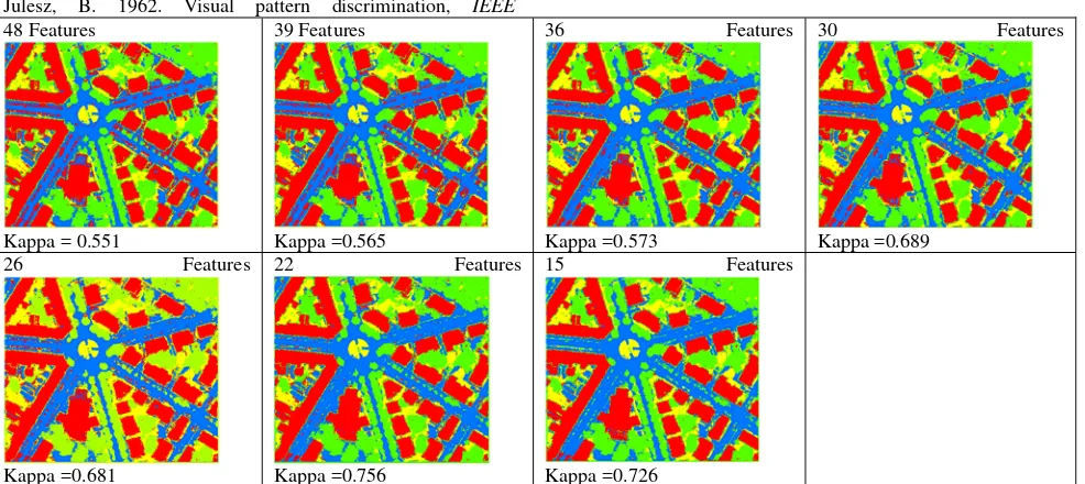
3.2 Feature selection results
To eliminate less important and more correlated features, iterative backward elimination scheme is used (Diaz-Uriarte and Alvarez de Andres, 2006). We first compute measures of feature importance to obtain an initial variable ranking and then proceed with an iterative backward elimination of the least important variables. In each iteration the least important
features (by default, 20%) are eliminated, and a new RF is built by training with the remaining features for the assessment of OOB errors based on OOB samples. The iterative procedure proceeds until the final features with the lowest OOB errors are determined for the land-use classification. In this study the number of trees (T) is set up 100-200, and the number of split variables is 4. Generally, the default setting of split variables is a good choice of OOB rate. Using OOB errors, the original 48 features are gradually eliminated up to 15 features. Meanwhile, as can be seen in Figure 4,the mean decrease accuracy is increasing with the decrease of numbers of features. The left fifteen features includes Lidar-NDVI, lidar height-based measures eigenvalue-Anistropy, nDSM, P-Normalized-Var, Height-Diff; Lidar intensity-based GLCM-Var., -Mean, and -SM; and aerial image-based GLCM-Homo and -Diss.
Figure 3. Random Forests-based feature importance
Figure 4. Iterative feature selection
4. CONCLUSIONS
In this study Random Forests is successfully applied to the feature selection for land-use classification. There are 48 features extracted from lidar data and imagery. Making use of the Random Forests, an assembling classification tree, that provides feature importance index, we iteratively eliminate features with less important index until the mean decrease accuracy is stable. The extensive experiments are conducted to describe the Random Forests’ characteristics and prove its performance. Classification results suggest that much more feature cannot guarantee the improvement of classification accuracy, and confirms that the selected features can obtain the satisfied classification results. Overall, the classification results indicate that the selected features agree the existing physiological knowledge.
REFERENCES
Arefi, H., Hahn, M., and Lindenberger, J., 2003. Lidar data classification with remote sensing tools, Proceedings of the ISPRS Commission IV Joint Workshop: Challenges in Geospatial Analysis, Integration and Visualization II, 08–09 September, Stuttgart, Germany, pp. 131–136.
Breiman, L., Friedman, H., Olshen, A. and Stone, J., 1984. Classification and Regression Trees. Monterey, CA: Wadsworth & Brooks/Cole Advanced Books & Software.
Breiman, L., 1996. Bagging predictors. Machine Learning, 24 (2), 123–140.
Breiman, L., 2001. Random Forests. Machine Learning, 45, 5– 32.
Chehata, N., Guo, L. and Mallet, C., 2009. Airborne lidar feature selection for urban classification using random forests. In: F. Bretar, M. Pierror-Deseilligny & G. Vosselman, eds. Laser Scanning, IAPRS, 38(3/W8). s.l.:s.n.
Congalton, G., 1991. A review of assessing the accuracy of classifications of remotely sensed data, Remote Sensing of Environment, 37(1): 35-46.
Congalton, G. and Green, K., 2009. Assessing the Accuracy of Remotely Sensed Data: Principles and Practices, Taylor & Francis, Boca Raton, FL. pp. 85-89.
Diaz-Uriarte, R., and Alvarez de Andres, S., 2006. Gene selection and classification of microarray data using random forest, BMC Bioinformatics, 7(3).
Gislason, P. O., Benediktsson, J. A. and Sveinsson, J. R., 2006. Random Forests for land cover classification, Pattern Recognition letters, 27:294-300.
Guo, L., Chehata, N., Mallet, C. and Boukir, S., 2011. 0
0.01 0.02 0.03 0.04 0.05 0.06
0.01
0.02
0.03
0.04
0.05
0.06
0.07
0.08
48
39
36
30
26
22
15
Mean Decrease
Accuracy
Relevance of airborne lidar and multispectral image data for urban scene classification using Random Forests, ISPRS Journal of Photogrammetry and Remote Sensing, 66(1): 56-66.
Haala, N. and Walter, V., 1999. Automatic classification of urban environments for database revision using lidar and color aerial imagery, International Archives of Photogrammetry and Remote Sensing, Vol. 32, Part 7-4-3 W6, Valladolid, Spain, 3-4 June, 1999.
Horning, N., 2010. Random Forests: An Algorithm for Image Classification and Generation of Continuous Fields Data Sets. Proceeding of International Conference on Geoinformatics for Spatial Infrastructure Development in Earth and Allied Sciences .
Jensen, J.R., 2005. Introductory Digital Image Processing, 3rd Ed. Prentice Hall, Upper Saddle River, N.
Joelsson, R., Benediktsson, A. and Sveinsson, R., 2008. Random Forest Classification of Remote Sensing Data. In: C. Chen, ed. Image Processing For Remote Sensing. Boca Racon, FL: CRC Press, pp. 61-78.
Julesz, B. 1962. Visual pattern discrimination, IEEE
Transaction on Information Theory, 8:84-92.
Perona P., and Malik, J., 1990. Scale-space and edge detection using anisotropic diffusion, IEEE Transactions on Pattern Analysis and Machine Intelligence, 12 (7): 629–639.
Stumpf, A. and Kerle, N., 2011. Object-oriented mapping of landsides using Random Forests, Remote Sensing of Environment, 115:2564-2577.
Wang, X., Waske, B. and Benediktsson, A., 2009. Ensemble Methods for Spectral-spatial Classification of Urban Hyperspectral Data. In Proceedings of IGARSS, Volume 4, pp. 944-947.
ACKNOWLEDGEMENTS
This study was financially supported by a NSERC discovery grant that was awarded to Prof. Dr. Jonathan Li at the University of Waterloo.
48 Features
Kappa = 0.551
39 Features
Kappa =0.565
36 Features
Kappa =0.573
30 Features
Kappa =0.689 26 Features
Kappa =0.681
22 Features
Kappa =0.756
15 Features
Kappa =0.726
Figure 5. the Maximum Likelihood classification results based on feature selection of Random Forests