CLASSIFICATION UNDER LABEL NOISE BASED ON OUTDATED MAPS
A. Maas, F. Rottensteiner, C. Heipke
Institute of Photogrammetry and GeoInformation, Leibniz Universit¨at Hannover, Germany -(maas, rottensteiner, heipke)@ipi.uni-hannover.de
Commission II, WG II/6
KEY WORDS:Supervised Classification, Label Noise, Logistic Regression, Map Updating
ABSTRACT:
Supervised classification of remotely sensed images is a classical method for change detection. The task requires training data in the form of image data with known class labels, whose manually generation is time-consuming. If the labels are acquired from the outdated map, the classifier must cope with errors in the training data. These errors, referred to as label noise, typically occur in clusters in object space, because they are caused by land cover changes over time. In this paper we adapt a label noise tolerant training technique for classification, so that the fact that changes affect larger clusters of pixels is considered. We also integrate the existing map into an iterative classification procedure to act as a prior in regions which are likely to contain changes. Our experiments are based on three test areas, using real images with simulated existing databases. Our results show that this method helps to distinguish between real changes over time and false detections caused by misclassification and thus improves the accuracy of the classification results.
1. INTRODUCTION
The updating of topographic databases (referred to asmapsfor brevity) is typically based on a classification of current remote sensing imagery. Comparing the results to the map, areas of change can be detected and the map can be updated accordingly. Supervised classification is commonly used for that purpose, re-quiring representative training data that are typically generated in a time-consuming manual process. The latter could be avoided by using the existing map to derive the class labels of the training samples. As the map may be outdated, classifiers using the class labels derived from the map for training must take into account the fact that some of these labels will be wrong. Nevertheless, changes typically only affect a relatively small part of a scene, so that one can assume the majority of the training data to be correct.
In machine learning, errors in the class labels of training data are referred to aslabel noise(Fr´enay and Verleysen, 2014). In remote sensing, the problem has mostly been dealt with by data cleans-ing, i.e. by detecting and eliminating wrong training samples, e.g. (Radoux et al., 2014). An alternative is to use probabilistic methods for training under label noise which also estimate the parameters of a noise model. An example for such an approach is the label noise tolerant logistic regression (Bootkrajang and Kab´an, 2012), which has been applied successfully in the context of remote sensing in (Maas et al., 2016). However, the underlying noise model of that technique assumes wrong labels to occur at random positions in the image. This is not a very realistic model for change detection, where changes typically occur in clusters, e.g. due to the construction of a new building, and may lead to a degradation of the classification performance.
Using the existing map has another potential benefit. As change is usually a rare event, the existing class labels can be seen as providing observations for the prediction of the new class labels. This may be particularly useful in areas where the classifier can-not distinguish the class label by the given features well, e.g. at object borders. The corresponding probabilities for the classes to be correct are related to the probability of observing a wrong
label and, thus, to the parameters of a probabilistic noise model (Bootkrajang and Kab´an, 2012). However, such an assumption again neglects the fact that changes typically occur in compact clusters. It would typically lead to a strong bias for maintain-ing the class label of the map, which is desired in areas without changes, but may limit the prospects of detecting real changes.
In this paper, we propose a new supervised classification method that tries to extract as much benefit as possible from the avail-ability of the existing map. Firstly, our method uses the class labels from the map for training. This is achieved by expanding the method by Bootkrajang and Kab´an (2012) to take into ac-count that changes typically occur in clusters, which we expect to improve the results in scenes with a large amount of change. Secondly, the class labels of the existing map are included as observations in a classification procedure based on Conditional Random Fields (CRF). We propose an iterative procedure to re-duce the impact of the observed class labels in compact areas that are likely to have changed, which we expect to improve the clas-sification results in areas of weak features without affecting the detection of real changes too much. For evaluation we use three data sets with different degrees of simulated changes.
2. RELATED WORK
Of the basic strategies for change detection identified in Jianya et al. (2008), we apply the one in which changes are inferred from differences between the independent classification of a current image and the existing map, because no sensor data are assumed to be available for the time of the acquisition of the existing map. Nevertheless, the existing map will be integrated into the classi-fication process, which is also the focus of this paper.
random(NAR) model, the probability of an error depends on the class label. If the dependencies between labelling errors and the observed data are considered, the model is callednoisy not at ran-dom(NNAR). This would be an appropriate choice in our case to model that label noise typically occurs in clusters in image space. We do not build a NNAR model explicitly, but we use one im-plicitly by an iterative strategy for reducing the impact of training samples forming clusters of potentially changed pixels. Existing NNAR models tend to analyse the distributions of the training samples in feature space, e.g. assuming label noise to occur more likely near the classification boundaries or in low-density regions (Sarma and Palmer, 2004). Apart from being drawn from another domain than image classification, this is not a model of local de-pendencies between label noise at neighbouring data sites.
Fr´enay and Verleysen (2014) distinguish three strategies for deal-ing with label noise. First, classifiers that are robust to label noise by design can be used, e.g. random forests, but they still may have difficulties with large amounts of label noise (Maas et al., 2016). The second strategy tries to remove training samples af-fected by label noise from the training set. Suchdata cleansing methods have been criticised for eliminating too many instances (Fr´enay and Verleysen, 2014). The third option is to use a classi-fier which is tolerant to label noise. In this context,probabilistic approacheslearn the parameters of a noise model along with the classifer in the training process; examples are (Bootkrajang and Kab´an, 2012), using logistic regression as the base classifier, and (Li et al., 2007), presenting a method based on the kernel Fisher discriminant. An example for anon-probabilistic approachis the label noise tolerant version of a Support Vector Machine (SVM) (An and Liang, 2013). However, non-probabilistic methods typ-ically do not estimate the parameters of a noise model, e.g. tran-sition probabilities containing the probability for the observed la-bel to be affected by a change (Bootkrajang and Kab´an, 2012), which may be used as temporal transition matrices in our appli-cation, linking the observed class labels of the map to class labels at the second epoch (Schistad Solberg et al., 1996).
In the domain of remote sensing, classification under label noise seems to be based on data cleansing in most cases. An example is (Radoux et al., 2014), who include two techniques for elimi-nating outliers to derive training data from an existing map. The first technique removes training samples near the boundaries of land cover types and the other one removes outliers based on a statistical test, assuming a Gaussian distribution of spectral sig-natures. Designed for data of 300 m ground sampling distance (GSD), the model assumptions, e.g. Gaussian distributions, can-not be used directly for high resolution images. A similar method was used for map updating in (Radoux and Defourny, 2010), us-ing Kernel density estimation for derivus-ing probability densities. Another data cleansing method is reported in (Jia et al., 2014). Similarly to the method proposed in this paper, all pixels from an existing map are used for training and the resulting label image is compared to the existing map to detect changes. However, no parameters of a model for label noise are estimated in the train-ing process. This is also true for the data cleanstrain-ing method based on SVM reported in (B¨uschenfeld, 2013), who eliminate training samples that are assigned to another class than indicated by the given map or that show a high uncertainty. Label noise tolerant training using maps for deriving training data was done by Mnih and Hinton (2012). They propose two loss functions tolerant to label noise to train a deep neural network, but their method only deals with binary classification problems. Bruzzone and Persello (2009) include information of the pixels in the neighbourhood of the training samples in the learning process to achieve
robust-ness to label noise in a context-sensitive semi-supervised SVM. Although the authors argue that such a strategy can be used to integrate existing maps for training, this is not shown explicitly.
In (Maas et al., 2016), we applied label noise tolerant logistic re-gression (Bootkrajang and Kab´an, 2012) to use an existing map for training, integrating it into a CRF for context-based classi-fication. The experiments showed that the method is tolerant to a large amount of label noise if it is randomly spread over the image, as would be expected for a method based on a NAR model. However, experiments with more realistic changes were only shown with a small percentage of wrong training labels, and the class labels from the existing map were not used in the clas-sification process. The latter was done by Schistad Solberg et al. (1996), who applied a temporal model based on transition prob-abilities to include an outdated land cover map in multitemporal classification, but no local dependencies between changes were considered. In this paper we want to expand our previous work (Maas et al., 2016) by considering the fact that changes occur in clusters. Label noise logistic regression Bootkrajang and Kab´an (2012) is applied in an iterative procedure in which the impact of training samples in areas of potential change is reduced, while these samples are not completely eliminated. To consider local context, the resultant classifier was integrated in a CRF, in which we also consider the original class labels as additional observa-tions. In contrast to (Schistad Solberg et al., 1996), the influence of these observations may change in the course of an iterative pro-cess if a pixel is situated in a large cluster of potentially changed pixels, so that temporal oversmoothing (Hoberg et al., 2015) can be avoided. Our method can be seen as a combination of ”soft” data cleansing (because samples are not eliminated completely) with a probabilistic noise model for including the observed labels from the map. Thus, we expect to be able to cope with a larger amount of real change than our previous method.
3. LABEL NOISE TOLERANT CHANGE DETECTION
We assume remotely sensed data and an existing but outdated raster map to be available on the same grid. The data consist of N pixels, each pixelnrepresented by a feature vectorxn =
[x1
n, ..., xFn]of dimension F, calculated from the imagery, and an observed class labelCen ∈ C = {C1, ..., CK}from the exist-ing map. Cdenotes the set of classes and K is the total
num-ber of classes. As the database may be outdated, the observed labels may differ from the unknown true labelsCn ∈ C. Col-lecting the observed and the unknown class labels in two vectors
e
C = (Ce1, ...,CeN)T andC = (C1, ..., CN)T, respectively, and denoting the observed image data byx, it is our goal to find the optimal configuration of class labelsCby maximising the joint posteriorP(C|x,Ce)of the unknowns given the observations. In this process, we use the class labels of the outdated map for de-riving the class labels of the training samples. We start by out-lining our modified version of the training procedure for logistic regression by Bootkrajang and Kab´an (2012) (Section 3.1). In Section 3.2, we show how logistic regression is integrated into a CRF (Kumar and Hebert, 2006) together with a model for con-sidering the existing class labelsCeas observations. Section 3.3 describes the new iterative procedure for training and inference.
3.1 Label noise robust logistic regression
A feature space transformationΦ(xn)may be applied to achieve non-linear decision boundaries in the original feature space. In the multiclass case the posterior is modelled by (Bishop, 2006):
p(Cn=Ck|xn) =
wherewk is a vector of parameters for a particular class Ck. As the sum of the posterior over all classes has to be 1, these parameter vectors are not independent, so thatw1is set to0; the other vectors are collected in a joint parameter vectorw.
In our case, each training sample consists of a feature vector xnand the observed labelCen. In order to consider this fact in training, Bootkrajang and Kab´an (2012) model the probability
p(Cen|xn)as the marginal distribution of the observed labelsCen over all values the unknown class labelsCnmay take:
p(Cen=Ck|xn) =
is the probability for a specific type of label noise affecting the two classesCaandCk. These
tran-sition probabilitiesfor all class configurations form the K x K transition matrixΓwithΓ(a, k) =γak=p(Ce=Ck|C=Ca). The transition matrixΓcontains the parameters of a NAR model which are estimated along with the parameterswin eq. 1. Be-cause this kind of model is unrealistic to describe changes in land cover, we introduce a weightgn ∈ (0...1]for every samplen to control its influence in the training process. In the beginning, these weights are all set to 1; Section 3.3.3 describes how they are changed iteratively to consider the assumption that changes occur in local spatial clusters. To deterimine the unknown param-eterswandΓ, we apply maximum likelihood estimation of the unknown parameters with a Gaussian prior overwfor regularisa-tion. Taking the negative logarithms of the involved probabilities, this results in the minimisation of the following target function:
E(w,Γ) =− and the rightmost term corresponds to a Gaussian prior with zero mean and covarianceσ·I, whereIis a unit matrix.
We use the Newton-Raphson method (Bishop, 2006) for minimis-ingE(w,Γ). In each iterationτ, the parameter vectorwτ
is determined fromwτ−1
according towτ = wτ−1− matrix, andδ(·)is the Kronecker delta function delivering a value of 1 if the argument is true and 0 otherwise.
Optimising for the unknown weights requires knowledge about the transition matrixΓ, which, however, is unknown. Bootkra-jang and Kab´an (2012) propose an iterative procedure similar to expectation maximisation (EM). Starting from coarse initial val-ues forΓ, the parameterswof the classifier are updated as just described. Using these weights, the transition matrixΓis updated afterwards, expanding the updating step presented in (Bootkra-jang and Kab´an, 2012) by the weightsgn:
γτ =1
This alternating update of the parameterswandΓis repeated un-til a termination criterion is reached. The estimated parametersw are related to a classifier delivering the posterior for the unknown current labelsCn, not the noisy labelsCen.
Note that this training with equal weightsgnwas already used in (Maas et al., 2016). In this paper this is just the case in the beginning of the training procedure. Note that the transition ma-trixΓonly represents the transition between the old database and the current labels in this initial step with equal weightsgn. If the weights of training samples in large clusters of potential changes are low (cf. Section 3.3.3), the majority of the samples affected by label noise will have a low impact on the result, so thatΓonly represents residual label noise of small local extents for which the NAR model is a sufficiently good approximation.
3.2 CRF considering the existing map
CRFs are graphical models consisting of nodes and edges that can be used to consider local context in a probabilistic classifi-cation framework (Kumar and Hebert, 2006). The nodes of the underlying graph represent random variables whereas the edges connect pairs of nodes and describe their statistical dependen-cies. Here, the unknown nodes correspond to the current labels
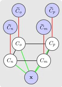
Cnof all pixelsn, and the edges are defined on the basis of a 4-neighbourhood on the image grid. As described above, the ob-served variables are the image dataxand, different from (Kumar and Hebert, 2006), the observed class labelsCe (cf. fig. 1 for the structure of the graphical model). The joint posteriorP(C|x,Ce) of the unknowns given the observations is modelled by:
P(C|x,Ce) = 1
wereZ is a normalization constant andǫis the set of edges in the graph. The association potentialAx(Cn,x)connects the un-known labelCnof pixelnwith the image datax. Its dependency from the entire input imagex is considered by using site-wise feature vectorsxn(x), which may be a function of certain im-age regions. Any discriminative classifier can be used to model this potential (Kumar and Hebert, 2006); here, it is based on the posteriorp(Cn|xn)of logistic regression according to eq. 1:
The interaction potentialI(Cn, Cm,x) describes the statistical dependencies between a pair of neighbouring labelsCnandCm. In this paper, the contrast-sensitive Potts model is used for that purpose, which results in a data-dependant smoothing of the re-sultant label image (Boykov et al., 2001):
I(Cn, Cm,x) =δ(Cn, Cm)·β0
β1+ 1−β1
·e
−∆x2
2σ2
D
,
(7) where the parametersβ0 andβ1 describe the overall degree of smoothing and the impact of the data-dependent term, respec-tively,σDis the average squared distance between neighbouring feature vectors,∆x=kxn−xmkis the distance of two feature vectorsxnandxm, andδ(·)is the Kronecker delta function.
The observed labels are related to the unknown class labels by the temporal association potentialAm(Cn,Cen), derived from the probability of the unknown label given the observed one:
Am(Cn,Cen) =θn·lnp(Cn=Ck|Cen=Ca) (8)
In eq. 8, there is an individual weightθn∈[0...1]for every pixel
n. This weight models the influence of the observed label on the classification result of this pixel in inference. As we shall see in Section 3.3, these weights will be adapted in the inference process to reduce the impact of the observed labels for pixels that are very likely to belong to a larger area affected by a change.
x
Co Cp
Cn Cm
e
Co Cep
e
Cn Cem
Figure 1. Graph structure of the expanded CRF:C: unknown labels,Ce: observed labels,x: image data.
3.3 Training and inference
In order to obtain the optimum configuration of the current class labels given the observations by maximisingP(C|x,Ce) accord-ing to eq. 5, a joint iterative trainaccord-ing and inference strategy is applied. After the determination of initial parameters of the asso-ciation potential and the parameters of the temporal assoasso-ciation potentials in an initial training phase, an iterative scheme of clas-sification and re-training is applied in which the weigths of pixels in large areas of potential change according to the current classi-fication result are modified to reduce their impact on the results. These steps are described in the subsequent sections.
3.3.1 Initial training and classification: In the initial train-ing phase, the observed labels and the data are used for label noise robust training of the logistic regression classifier that serves as the basis for the association potentials of the CRF. For that pur-pose, the method described in Section 3.1 is applied, using iden-tical weightsgn = 1for all training samples. This will result in an initial set of parameters w for the association potentials
and a transition matrixΓthat contains the transition probabilities
p(Cen = Ca|Cn = Ck)of the NAR model (Bootkrajang and Kab´an, 2012). According to the theorem of Bayes, these prob-abilities are related to the probprob-abilitiesp(Cn =Ck|Cen =Ca) required for the temporal association potential (eq. 8) by:
p(Cn=Ck|Cen=Ca) =
p(Cen=Ca|Cn=Ck)·p(Cn=Ck)
p(Cen=Ca)
As we have no access to the distribution of the unknown class labelsp(Cn), we assumep(Cn=Ck)≈p(Cen=Ck)to derive the temporal association potential fromΓ. These parameters are kept constant in the subsequent iteration process for the reasons already pointed out in Section 3.1: the transition matrix corre-sponds to the real transition probabilities only in the first iteration (when all training samples have an identical weightgn= 1). The parameters of the interaction potentials (β0, β1; cf. eq. 7) are set to values found empirically.
For the determination of the optimal configuration of labelsC= argmax(P(C|x,Ce))loopy belief propagation is used (Frey and MacKay, 1998). In the initial classification, the weightsθnof the temporal association potentials is set to 0 for all pixels, so that this classification is only based on the current state of the association and the interaction potentials.
3.3.2 Iterative re-training and classification: By comparing the current label image with the outdated map, areas of potential changed areas can be detected. This information is used to up-date the weightgnof each training sample, and label noise robust training of the logistic regression classifier is repeated, using the updated weights. The way in which the weights are updated is explained in Section 3.3.3. Training will result in new values for the parameterswof the association potentials of the CRF.
Furthermore, the information about potential areas of change is also used to change the weightsθnof the temporal association potentials as explained in Section 3.3.4. Using the updated pa-rameterswand weightsθn, another round of inference is carried out, which will lead to an improved classification result. This procedure of updating weights on the basis of the current state of the classification results, re-training and inference is repeated until the proportion of weights that are changed in an iteration is below a threshold or a maximum number of iterations is reached. The procedure is inspired by re-weighting strategies for robust es-timation in adjustment theory, e.g. (F¨orstner and Wrobel, 2016).
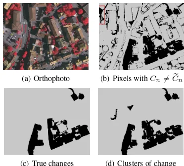
3.3.3 Weightsgnof training samples: The weightgnof a training samplenshould be high for samples which are probably not affected by a change and low for other ones. The weights are initialised bygn = 1as long as no information about changes is available. After classification, the resulting labelsCncan be compared to the mapCen to generate a binary mapBC of po-tential changes. However, as indicated in fig. 2(b) for an aerial image, this binary map will also contain classification errors.
cer-tain minimum size. This is considered by removing all con-nected components of foreground pixels inBC which cover an area smaller than a thresholdu. The third assumption is that in areas affected by cast shadows, the quality of spectral information or of the DSM (if available) is poor and, thus, potential changes as indicated byBCare very likely to correspond to classification errors. To detect shadow areas, the median and the mean of the image intensity in each clusterclis compared to the median and the mean of the entire images. Ifmeancl < meanimg/2and
medcl < medimg/2, i.e., if the pixels in the cluster are very dark compared to the image, the pixels belonging to clusterclare removed from the binary map of potential changesBC. The re-maining foreground pixels inBCare likely to correspond to real changes (cf. fig. 2(d) for an example).
For pixels corresponding to the foreground inBC, the weightsgn are decreased by a constantc, so that in iterationt+ 1, the weight of the corresponding samples is given bygt+1
n =max(gnt−c, ξ). The minimal weight is set to a small constantξto avoid numerical problems. The weights of pixels that belong to the background inBC are updated according tognt+1 = min(gnt +c,1). As a consequence, the weights of pixels that are considered to be changes will be reduced in each iteration; however, a pixel may regain influence if in a certain iteration its most likely class label is identical to the one from the map, e.g. due to the influence of its neighbours or due to the temporal model.
(a) Orthophoto (b) Pixels withCn6=Cen
(c) True changes (d) Clusters of change
Figure 2. Example for the identification of potential areas of change. Black / gray: changed / unchanged pixels. Red rectangle in (b): a cluster that corresponds to a shadow.
3.3.4 The weightsθnof the temporal association potential: The weightθnof pixelnregulates the impact of the temporal association potential and, thus, the influence of the outdated map to the resulting label configurationC (cf. eq. 8). If a pixel is probably not affected by a change, the weightθnshould be high, otherwise it should be low. The initial weight for each pixel is 0, because in the beginning we do not want to bias the result to reject potential changes. In the subsequent iterations, the binary map of potential changes used to adapt the weightsgn of the training samples (cf. Section 3.3.3) is also used to guide the adaptation of the weightsθnof the temporal model, because the same assump-tion w.r.t. to the plausibility of a potential change indicated by the current classification results apply. In iterationt+1, the temporal association potentials for pixels corresponding to the foreground inBC will the be weighted byθtn+1 = max(θtn−c,0). The corresponding weights of pixels that belong to the background in
BCare updated byθnt+1=min(θtn+c,1).
4. EXPERIMENTS
4.1 Test data and test setup
We used three datasets in our experiments. The first one consists of a part of Vaihingen data of the ISPRS 2D semantic labelling contest (Wegner et al., 2015). We use ten of the training patches, each consisting of about 2000×2500 pixels. For each patch, a colour infrared true orthophoto (TOP) and a DSM are avail-able with a ground samling distance (GSD) of 9 cm. The refer-ence consists of five classes:impervious surfaces(sur.),building (build.),low vegetation(veg.),tree, andcar. As cars are not a part of a topographic map, this class was merged withsur. For each pixel, we defined a feature vectorxn(x)consisting of the normalised difference vegetation index (NDVI), the normalised DSM (nDSM), the red band of the TOP smoothed by a Gaussian filter withσ= 2, and hue and saturation obtained from the TOP, both smoothed by a Gaussian filter withσ= 10. These features were selected from a larger pool based on the feature importance analysis of a random forest classifier (Breiman, 2001).
The other two data sets are based on satellite imagery and were also used in in (Maas et al., 2016). The first one consists of a Landsat image from 2010 of an area near Herne, Germany, with a GSD of 30 m and a size of 362×330 pixels. The second dataset consists of a RapidEye image of an area near Husum, Germany, from 2010. Its GSD is 5 m and its size is 3547×1998 pix-els. In both cases only the red, green and near infrared bands are available. The reference contain four classesresidential area (res.),rural streets, forest(for.) and cropland(crop.). As the classrural streetsis underrepresented in both images, we merged it withcropland. In both datasets, 19 features were selected: four Haralick features (energy, contrast, homogenity and entropy) re-lated to texture, the mean and variance of five spectral features (near infrared band,intensity,hue,saturationandndvi) in a lo-cal neighbourhood of 6×6 pixels and the values of the same spectral features smoothed by a Gaussian filter withσ= 5.
For Vaihingen, we used a feature space mappingΦ(xn)based on quadratic expansion, whereas for Husum and Herne no fea-ture space mapping was used. The hyperparameter for regular-isation in eq. 3 was set to σ = 10. The initial values for the transition matrixΓ(cf. Section 3.1) wereγij = 0.8fori =j andγij = 0.2/(K−1)fori6= j, whereKis the number of classes. The initial values for the parameter vectorwof logistic regression were determined by standard logistic regression train-ing without assumtrain-ing label noise. The parameters of the contrast-sensitive Potts model were set toβ0 = 1.0andβ1 = 0.5. The thresholds for updating the weights (Section 3.3.3) depend on the GSD. For Vaihingen, the threshold for object bordersswas set to 0.5 m, assuming wrong classifications near object borders to be caused by errors in the nDSM or mixed pixels. The minimal sizeuof an object is set to 4 m×4 m (i.e., smaller than a small house). For the satellite data,sis set to 2 pixels, because mis-takes caused by the nDSM do not exist, anduis set to 250 m×
250 m, assuming this is the minimum size of a new residential area or field. The valuecfor updating the weights (Sections 3.3.3 and 3.3.4) was found empirically and set to0.1. Except for the dataset of Herne, where all pixels are used due to the small image size, just about 20% of the data are used for training to reduce the processing time. The iteration is terminated (Section 3.3.2) if either less than 0.01% of the weights for the observed labels in classification change or if at least 40 iterations have been done.
three simulated maps were created, each with a different amount of change. For Herne and Husum, the changed map from (Maas et al., 2016) were used. Based on these data, we carried out four experiments. In the first experiment (Init), training and classifi-cation was carried out as in (Maas et al., 2016), i.e. without iter-ative re-training and classification(gn= 1 =const, θn= 0 =
const). The second experiment (Vg) is based on our method, but without considering the outdated map(θn= 0 =const). It shows the impact of the sample weightsgnintroduced in section 3.1 in the training step. The third experiment (Vθ) uses constant training weightsgn = 1, but does apply the modified weights
θnto include the map information. The last experiment, Vgθ, uses our method with weight modification both in the training and classification steps. In each case, we compare the results to the reference on a per-pixel basis, determining the overall accuracy (OA) as well as completeness and correctness per class (Heipke et al., 1997). Comparing the simulated map with the real refer-ence shows the amount of change in the corresponding data set, and the resultant quality indices are also reported (map); 100% -OA ofmapgives the amount of simulated change in each exper-iment. We do not distinguish a training set from a test set because an outdated map is always used, at least for training.
4.2 Results and evaluation
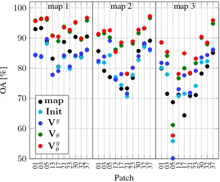
4.2.1 Vaihingen: Fig. 3 shows the OA of all patches achieved for three versions of the outdated map (map 1 – map 3) for Vai-hingen. In most cases the variantVθgachieves the best OA (85%-90%), but variantVθperforms at a similar level, and both vari-ants clearly outperform the varivari-ants without weights and without considering the outdated map (Init,Vg). Obviously, the inclu-sion of the outdated map has a relatively high impact on the qual-ity of the results, improving the OA by 2%-10%. This is mainly caused by an improved classification at object boundaries or at individual pixels. In fact, in some cases, the variants not consid-ering the outdated map lead to results where a larger percentage of change than actually present is predicted, so that the corre-sponding OA is lower than the one indicated bymap.
01 03 05 13 17 21 23 30 32 37 01 03 05 13 17 21 23 30 32 37 01 03 05 13 17 21 23 30 32 37
50 60 70 80 90
100 map 1 map 2 map 3
Patch
O
A
[%]
map Init
Vg Vθ Vgθ
Figure 3. Overall accuracy for the four variants in Vaihingen.
The advantage of considering the sample weightsgnin training becomes more obvious for experiments with a large amount of change. If the level of change is small, it can be compensated by the original method based on the NAR model (Maas et al., 2016). If the label noise cannot be compensated by the NAR model any more, considering the weights can improve the results.
One example is patch 17 (fig. 4). It contains three buildings with a brighter appearance than the rest (blue rectangles in fig. 4(a)). Only one of them is contained in the outdated map (fig. 4(b)). Without considering the weights (variant Init, fig. 4(c)), one building is mostly classified asveg. In variantVgthe two changed buildings are correctly detected (fig. 4(d)). Another difference between the results of variantsInitand Vg is the label of the vineyard which belongs to the classveg.but is often classified as treein experimentInit. Without considering weights, the proba-bilityp(Cn|xn)is low for all classes in the area of the vineyard, so that the classification results are not reliabe. By considering the sample weights in experimentVg, the probabilityp(C
n|xn) for the classveg.is much higher than for the other classes. How-ever, because the vineyard has a similar appearance to trees, the tree marked in fig. 4(c) is also classified asveg.inVg
.
(a) Orthophoto (b) Outdated map 3
(c)Init (d)Vg
Figure 4. Data and results from patch 17 (Vaihingen). Red: build., dark green:tree, light green:veg., gray:sur.. Blue
rectangles: highlighted objects discussed in the text.
For patch 5 (fig. 5) and the otudated map 3 with more than 30% label noise, OA is always below 61% (fig. 3). In this case nearly 50% of all building pixels are labeled assur.in the outdated map. This amount of label noise cannot be dealt with by the original method (Init). The transition probabilitiesγiifor no change for build.andsur.determined in the initial training step are close to 1 and, thus, not very accurate. Consequently, the iterative weight updating procedure does not converge to the correct solution.
(a) Orthophoto (b) map 3 (c)Init (d)Vg θ
Figure 5. Data and results from patch 5 (Vaihingen). Red:build., dark green:tree, light green:veg., gray:sur.
Figs. 6 and 7 show the completeness and the correctness of the re-sults. Both quality indices are higher for variantsVθandVθgthan for the others, which again highlights the importance of using the outdated map for classification. Using the sample weightsgnin the training process does not improve the completeness in most cases, but it does have a small positive impact on the correctness.
b
uild. tree veg. sur
.
b
uild. tree veg. sur
.
b
uild. tree veg. sur
.
60 70 80 90
100 map 1 map 2 map 3
Class
Completeness
[%]
map Init
Vg Vθ Vgθ
Figure 6. Average completeness over all patches in Vaihingen.
b
uild. tree veg. sur
.
b
uild. tree veg. sur
.
b
uild. tree veg. sur
.
60 70 80 90
100 map 1 map 2 map 3
Class
Correctness
[%]
map Init
Vg Vθ Vgθ
Figure 7. Average correctness over all patches in Vaihingen.
were excluded from the evaluation. The mean completeness and correctness of all areas are shown in tab. 1. Again, variantVgθ achieves the best completeness (98.9%) and correctness (82.5%). However, variantsVθandVg
do not perform significantly worse considering the standard deviations of the quality indices. Never-theless one can notice an positive impact of the new developments presented in this paper (variantsVg,Vθ and, particularly,Vθg) compared to the original algorithm (Init) (Maas et al., 2016).
Vθg Vθ Vg Init map
Corr. 99 [4] 99 [4] 96 [8] 93 [14] 91 [11] Compl. 82 [19] 80 [17] 82 [18] 75 [20] 74 [13]
Table 1. Completeness and correctness on a per-object basis for buildings; mean of all areas in % [standard deviation in %]
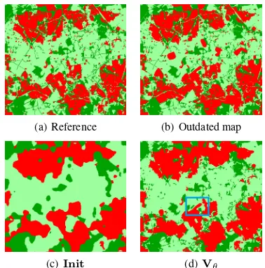
4.2.2 Herne and Husum: As the amount of change in Husum and Herne is quite small (3% - 4%), using the sample weightsgn does not affect the results much; the OA changes by less than 0.6%. Thus, this section focuses on the impact of using the out-dated map for classification. In tab. 2 OA, completeness and cor-rectness are shown for both datasets for variantsInitandVθ. All values are larger for variantVθ by a large margin, the OA increasing by 13.9% for Herne and by 5.2% for Husum. One reason for that increase is the improvement of the delineation of object borders. As the features all depend on a local subset of pixels, borders of objects are blurred in the standard classifica-tion process. In variantVθthese areas can be correctly classified in regions without change. If regions of change are smaller than the thresholdu(Section 3.3.3), considering the map has the same effect, which may lead to cases in which such small changes are not detected. An example for such a situation in Herne with
vari-antVθ is indicated by a blue rectangle in fig. 8(d). To highlight the potential for detecting changes despite using the existing map for classification, tab. 3 shows the OA achieved for pixels in the areas affected by a change. The results show that the improved OA for the entire image caused by the inclusion of the outdated map (cf. tab. 2) comes at the cost of a reduced OA in the changed areas. In Husum, this reduction in OA is low (0.8%). In Herne it is somewhat larger (7%), though still considerably smaller than the improvement for the entire scene (14.4%).
(a) Reference (b) Outdated map
(c)Init (d)Vθ
Figure 8. Label images for Herne. Dark green: forest, light green:crop., red:res.. Blue rectangle: an undetected change.
Dataset Herne Herne Husum Husum
Vθ Init Vθ Init
OA 89.7 75.8 96.7 91.5
res. 95.7 83.4 88.7 79.3
Compl. for. 76.8 54.9 91.5 77.7
crop. 92.4 81.6 98.2 94.4
res. 81.2 74.3 87.5 72.2
Corr. for. 96.7 69.7 92.2 75.2
crop. 93.8 79.4 98.3 95.9
Table 2. OA, completeness, correctness for Husum and Herne.
Herne,Init Herne,Vθ Husum,Init Husum,Vθ
75.9 % 68.9 % 92.6 % 91.8 %
Table 3. OA of Husum and Herne for areas affected by a change.
5. CONCLUSION AND FUTURE WORK
We tested our method using datasets with different properties and varying degrees of label noise. Due to our re-weighting scheme for training samples the method can also deal with larger amount of noise, but the improvement brought about by this strategy was smaller than expected. The inclusion of the map information to the CRF has a considerably larger positive effect, largely due to a better classification of pixels near object boundaries. The actual changes are detected nearly as good as without considering the map in classification, although very small changed objects might not be detected. These observations could be made independently from the GSD of the images. A major limitation of the method is that each cluster in feature space still must contain enough correct training samples for it to work. If the results of the base classi-fier in the initialization step are sufficiently good, considering the map in the classification can improve the results considerably.
In our future work we want to expand our model by images from other epochs, so that not only the map can help to improve the classification result, but also other image data. Additionally we want to expand our experiments to data with real changes to see how our method works under more realistic circumstances in terms of the extent of change, level of detail or number of classes.
ACKNOWLEDGEMENTS
This research was funded by the German Science Foundation (DFG) under grant HE-1822/35-1. The Vaihingen data set was provided by the German Society for Photogrammetry, Remote Sensing and Geoinformation (DGPF) (Cramer, 2010):
http://www.ifp.uni-stuttgart.de/dgpf/DKEP-Allg.html.
REFERENCES
An, W. and Liang, M., 2013. Fuzzy support vector machine based on within-class scatter for classification problems with outliers or noises.Neurocomputing110, pp. 101–110.
Bishop, C. M., 2006.Pattern recognition and machine learning. 1st edn, Springer. New York (NY), USA.
Bootkrajang, J. and Kab´an, A., 2012. Label-noise robust logistic regression and its applications. In: Joint European Conference on Machine Learning and Knowledge Discovery in Databases, Springer, pp. 143–158.
Boykov, Y., Veksler, O. and Zabih, R., 2001. Fast approximate energy minimization via graph cuts. IEEE Transactions on pat-tern analysis and machine intelligence23(11), pp. 1222–1239. Breiman, L., 2001. Random forests. Machine learning45(1), pp. 5–32.
Bruzzone, L. and Persello, C., 2009. A novel context-sensitive semisupervised svm classifier robust to mislabeled training sam-ples. IEEE Transactions on Geoscience and Remote Sensing 47(7), pp. 2142–2154.
B¨uschenfeld, T., 2013. Klassifikation von Satellitenbildern unter Ausnutzung von Klassifikationsunsicherheiten. PhD thesis, Fortschritt-Berichte VDI, Reihe 10 Informatik / Kommunikation, Vol. 828, Institute of Information Processing, Leibniz Universit¨at Hannover, Germany.
Cramer, M., 2010. The DGPF-test on digital airborne cam-era evaluation – overview and test design. Photogrammetrie-Fernerkundung-Geoinformation2010(2), pp. 73–82.
F¨orstner, W. and Wrobel, B. P., 2016. Robust estimation and outlier detection. In:Photogrammetric Computer Vision, 1stedn, Springer, Cham, Switzerland, chapter 4.7, pp. 141–159.
Fr´enay, B. and Verleysen, M., 2014. Classification in the presence of label noise: a survey. IEEE transactions on neural networks and learning systems25(5), pp. 845–869.
Frey, B. J. and MacKay, D. J., 1998. A revolution: Belief prop-agation in graphs with cycles. Advances in neural information processing systems10, pp. 479–485.
Heipke, C., Mayer, H., Wiedemann, C. and Jamet, O., 1997. Evaluation of automatic road extraction. In: International Archives of Photogrammetry and Remote Sensing, Vol. XXII-3/4W2, pp. 151–160.
Hoberg, T., Rottensteiner, F., Feitosa, R. Q. and Heipke, C., 2015. Conditional random fields for multitemporal and multiscale clas-sification of optical satellite imagery.IEEE Transactions on Geo-science and Remote Sensing53(2), pp. 659–673.
Jia, K., Liang, S., Wei, X., Zhang, L., Yao, Y. and Gao, S., 2014. Automatic land-cover update approach integrating iterative train-ing sample selection and a markov random field model. Remote Sensing Letters5(2), pp. 148–156.
Jianya, G., Haigang, S., Guorui, M. and Qiming, Z., 2008. A re-view of multi-temporal remote sensing data change detection al-gorithms. In:The International Archives of the Photogrammetry, Remote Sensing and Spatial Information Sciences, Vol. XXXVII-B7, pp. 757–762.
Kumar, S. and Hebert, M., 2006. Discriminative random fields. International Journal of Computer Vision68(2), pp. 179–201. Li, Y., Wessels, L. F., de Ridder, D. and Reinders, M. J., 2007. Classification in the presence of class noise using a probabilis-tic kernel fisher method. Pattern Recognition40(12), pp. 3349– 3357.
Maas, A., Rottensteiner, F. and Heipke, C., 2016. Using label noise robust logistic regression for automated updating of topo-graphic geospatial databases. In:ISPRS Annals of Photogramme-try, Remote Sensing and Spatial Information Sciences, Vol. III-7, pp. 133–140.
Mnih, V. and Hinton, G. E., 2012. Learning to label aerial im-ages from noisy data. In:Proceedings of the 29th International Conference on Machine Learning (ICML-12), pp. 567–574. Radoux, J. and Defourny, P., 2010. Automated image-to-map discrepancy detection using iterative trimming.Photogrammetric Engineering & Remote Sensing76(2), pp. 173–181.
Radoux, J., Lamarche, C., Van Bogaert, E., Bontemps, S., Brock-mann, C. and Defourny, P., 2014. Automated training sample extraction for global land cover mapping. Remote Sensing6(5), pp. 3965–3987.
Sarma, A. and Palmer, D. D., 2004. Context-based speech recog-nition error detection and correction. In: Proceedings of HLT-NAACL 2004: Short Papers, Association for Computational Lin-guistics, pp. 85–88.
Schistad Solberg, A. H., Taxt, T. and Jain, A. K., 1996. A Markov random field model for classification of multisource satellite im-agery. IEEE Transactions on geoscience and remote sensing 34(1), pp. 100–113.