MAPPING UNDERSTORY TREES USING AIRBORNE
DISCRETE-RETURN LIDAR DATA
I. Korpela a,, A. Hovi a, F. Morsdorf b a
Department of Forest Sciences, POB 27, 00014 Univ. of Helsinki, Finland - (ilkka.korpela, aarne.hovi)@helsinki.fi b
Remote Sensing Laboratories, Dept. of Geography, Univ. of Zurich, Switzerland - [email protected]
Commission III
KEY WORDS: small-footprint, transmission loss, canopy gap, silviculture, forest inventory
ABSTRACT:
Understory trees in multi-layer stands are often ignored in forest inventories. Information about them would benefit silviculture, wood procurement and biodiversity management. Cost-efficient inventory methods for the assessment of the presence, density, species- and size-distributions are called for. LiDAR remote sensing is a promising addition to field work. Unlike in passive image data, in which the signals from multiple layers mix, the 3D position of each hot-spot reflection is known in LiDAR data. The overstory however prevents from obtaining a wall-to-wall sample of understory, and measurements are subject to transmission losses. Discriminating between the crowns of dominant and suppressed trees can also be challenging. We examined the potential of LiDAR for the mapping of the understory trees in Scots pine stands (62°N, 24°E), using carefully georeferenced reference data and several LiDAR data sets. We present results that highlight differences in echo-triggering between sensors that affect the near-ground height data. A conceptual model for the transmission losses in the overstory was created and formulated into simple compensation models that reduced the intensity variation in second- and third return data. The task is highly ill-posed in discrete-return LiDAR data, and our models employed the geometry of the overstory as well as the intensity of previous returns. We showed that even first-return data in the understory is subject to losses in the overstory that did not trigger an echo. Even with compensation of the losses, the intensity data was deemed of low value in species discrimination. Area-based LiDAR height metrics that were derived from the data belonging to the crown volume of the understory showed reasonable correlation with the density and mean height of the understory trees. Assessment of the species seems out of reach in discrete-return LiDAR data, which is a drastic drawback.
1. INTRODUCTION
Commercial forests in Finland are typically even-aged. Pine, spruce, and birch are the main species. A layer of shade-tolerant trees emerges commonly under pine and birch in ca. 10% of productive forest in southern Finland. Information of understory trees is of relevance for forest management.
Remote sensing was applied to understory vegetation (Eriksson et al. 2006; Peltoniemi et al. 2005; Korpela 2008). In passive optical data, the signals from the over and understory are mixed, which hampers the interpretation. Diffuse light, shading and occlusions are inherent properties of the understory. In this respect airborne LiDAR sensors offer a promising alternative. They illuminate the target and measure the travel time of very short pulses that can penetrate the canopy through gaps and reflect from several targets. The back-scattered photons are measured in shadow-free view-il-lumination geometry at low scan zenith angles. A discrete-return (DR) LiDAR extracts 1-4 echoes, while full-waveform LiDAR sensors sample and store the amplitude of the returning photon surge at high frequency. A measurable signal is not always obtained from below dense canopies due to transmission losses, since the energy is concentrated into a narrow cone, typically 0.1–0.5 m in diameter. The at-target energy decreases with increasing range, which decreases the SNR. Consequently, fewer echoes are detected from higher altitudes. Reflective but small targets not always scat-ter an adequate amount of photons to trigger an echo. However, even these weak interactions contribute to transmission losses, which complicate the interpretation of radiometric signals from the understory. DR sensors record the range and intensity, and intensity is assumed to correspond to the peak backscatter amplitude. Given a homogenous overstory, intensity is a potential measure of trans-mission losses except for volumetric reflections. The intensity observations are not physical entities, and sensors may differ in how the backscattered signal is interpreted into an echo. Thus, calibration using in situ reference data is likely needed in understory inventories as well.
The spatial pattern of understory trees, species composition, density and height (h) are important parameters for forestry. LiDAR point h- and intensity distribution metrics were used to characterize multiple canopy layers (Maltamo et al. 2005; Martinuzzi et al. 2009; Hill et al. 2009; Morsdorf et al. 2010). Research done in seedling stands shows that the accuracy of LiDAR in measuring and classifying small trees is limited (Korpela et al. 2008). Results in LiDAR-based tree species classification also suggest that the intensity data are noisy (Ørka et al. 2009).
A challenge in using h-distributions is the vertical overlap of the under and overstory trees. A further challenge is the represen-tativeness of the pulse sample that reaches the understory. The pulse pattern may provide a biased sample. Intensity data in DR systems could potentially be used for discriminating between tar-gets of different reflectance, structure and geometry. The noise due to transmission losses must however be accounted for. This is ill-posed in DR data, because of the losses due to weak and volumetric reflections, which are incompletely described by the intensity observations. The fact that intensity not only depends on target reflectance contributes to the ill-posed nature. DR systems have a blind zone of 1–4 m that follows an echo. These losses are not seen in the intensity data. The echo-triggering probability, intensity and transmission losses depend also on the geometry of the pulse–target intersection due to the uneven energy distribution within footprints. Our overall aim was to explore the potential of LiDAR in mapping understory trees for forestry applications. Using carefully measured in situ data we examined the basic relationships. We focused on the analysis of intensity data for tree species discrimination, which is an important practical aspect.
2. MATERIALS
2.1 Hyytiälä study area, field plots and measurements
The study was conducted in southern Finland in two pine-dominated stands (Table 1). Plot A is in a 50-year-old stand on
moraine soil. The understory consists mainly of downy birch and spruce. The plot contains a gradient in both site fertility and in the density of the understory. The bottom flora is characterized by 20– 50-cm-high bilberry, stem moss and wood moss. Plot B is located 4 km SSW from A, and has mature, 110-yr-old trees. It is located on sandy alluvial deposit with flat topography. The understory consists mainly of spruce and the twig layer of bilberry and lingonberry is sparse. Stem moss and fork mosses comprise the bottom layer.
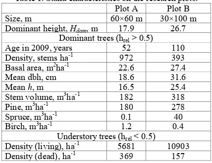
Table 1. Stand characteristics on the research plots. Plot A Plot B
Size, m 60×60 m 30×100 m
Dominant height, Hdom, m 17.9 26.7
Dominant trees (hrel > 0.5)
Age in 2009, years 52 110
Density, stems ha-1 972 393
Basal area, m2ha-1 22.6 27.4
Mean dbh, cm 18.6 31.6
Mean h, m 16.5 25.4
Stem volume, m3ha-1 182 318
Pine, m3ha-1 180 278
Spruce, m3ha-1 0.1 40
Birch, m3ha-1 1.2 0.4
Understory trees (hrel < 0.5)
Density (living), ha-1 5681 10903
Density (dead), ha-1 369 157
We aimed at positioning accuracies of 0.25 m and 0.15 m for the over and understory trees, respectively. A method was developed, which combined photogrammetry with field triangulation and trilateration. All photo-visible trees were positioned in aerial images using monoplotting in the LiDAR point clouds. The sX and
sY for the tree stems were 0.25 m on plot B (redundant intertree distance measurements). Mapping of understory followed in 6- 8-m-wide strips. A cable was tightened between two trees, which we-re positioned by trilateration-triangulation and adjustment of 8 distance, azimuth and XY coordinate observations, giving precision of 0.1 m. The position of trees with h > 0.3 m was derived by measuring the distance along the cable and perpendicularly to it using a large right-angle tool. A two-person crew measured 260 trees per day. The accuracy was controlled by mapping the photo trees with the cable method. sXYcable were 0.06-0.13 m. Redundant distances were measured between understory trees on plot B and contrasted to the calculated distances. Within-strip sXYcable were < 0.05 m, while between-strip sXYcable were 0.07 m. All trees were measured for h. The dbh and h of the crown base (hc) were
measured for the overstory trees. The h-distributions were bimodal (Fig. 1). The spatial pattern of the understory was uneven on both plots (Fig. 2). The mean h or density of the understory trees was tested spatially independent of the overstory trees at close distan-ces.
2.2 LiDAR data
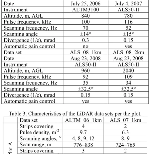
Four data sets from three campaigns were used (Table 2, 3). Sensors recorded 1-4 echoes per pulse and the trajectory data was included. The weather of June 2007 was very rainy and the last rain (6.4 mm) occurred only two days prior to the campaign. We used for illustrations LiDAR data from August 2004 and July, 2010. The XY accuracy of the LiDAR data was better than 0.25 m in photo-grammetric targets. The elevation accuracy was evaluated at Network-GNSS points and campaign-level offsets of below 6 cm were observed. In ALTM3100 data, raw observed intensities were normalized for range variation using an average reference range:
raw a
ref
corr I
R R
I ×
÷÷ø ö ççè æ
= (1)
In ALS50-II data, corrections for both R and AGC values were made using an empirical correction (Korpela 2008; Korpela et al. 2010):
(
c AGC)
I b I R
R
I raw raw
a
ref
corr × + × ×
-÷÷ø ö ççè æ
= (2)
Parameters b and c in Eq. 2 were solved using an F-test for intensity observations representing homogenous natural and artificial targets. The value of a was 2.4 in Eq. 1 and 2.5 in Eq. 2. They are compromises for forest canopies (Korpela et al., 2010). DEMs in a 0.5-m grid were estimated using the different LiDAR data sets with TerraScan software.
Fig. 1. h-distributions of trees in plots A and B. 3. METHODS
3.1 Geometric modelling of trees
To study LiDAR pulse-tree interaction, we geometrically modelled the reference trees. We confined ourselves to simple objects and the trees comprised of rotationally symmetric solids: a curve of revolution for the upper part of the crown, a cylinder for the lower part of deep crowns and a truncated cone for the stem.
Fig. 3 shows a pulse penetration map that was drawn at the mean crown base height (HC) the overstory. The map shows the autocorrelation of penetration and overstory. Such maps were drawn on a mapping surface at h = HC above the DEM, by back-projecting pulses to this h.
Fig. 2. Map of trees on plot A (left) and B (right). The symbol size for upper layer trees depicts hrel. Coordinates are in
meters (KKJ-2 system).
Table 2. Sensor configurations in the LiDAR data sets.
Data set ALTM_06_1km ALS_07_1km
Date July 25, 2006 July 4, 2007
Instrument ALTM3100 ALS50-II
Altitude, m, AGL 840 780
Pulse frequency, kHz 100 116
Scanning frequency, Hz 70 52
Scanning angle ±14° ±15°
Divergence (1/e), mrad 0.3 0.15
Automatic gain control no yes
Data set ALS_08_1km ALS_08_2km
Date Aug 23, 2008 Aug 23, 2008
Instrument ALS50-II ALS50-II
Altitude, m, AGL 960 2040
Pulse frequency, kHz 92 109
Scanning frequency, Hz 35 34
Scanning angle ±32.5° ±32.5°
Divergence (1/e), mrad 0.15 0.15
Automatic gain control yes yes
Table 3. Characteristics of the LiDAR data sets per the plot.
Data set ALTM_06_1km ALS_07_1km
Strips covering 4 2
Pulse density, m-2 9.7 6.3
Scanning angles, ° 4, 8, 9, 12 8, 9 Scan range, m 776-838 724-765
Strips covering 3 2
Pulse density, m-2 5.7 6.1
Scanning angles, ° 13.6, 8.2, 5.6 10.6, 5.9
P
lot
A
Scan range, m 827-921 765-805
Data set ALS_08_1km ALS_08_2km
Strips covering 2 2
Pulse density, m-2 2.1 0.9
Scanning angles, ° 6, 3 13, 12 Scan range, m 878-908 1881-1924
Strips covering 3 3
Pulse density, m-2 4.9 2.3
Scanning angles, ° 25.8, 25.1, 30.0 24.6, 23.9, 24.7
P
lot
B
Scan range, m 1003-1102 2059-2130 3.2 Pulse-target geometric analyses
An analysis procedure was developed to study pulse-tree intersections, using the geometric tree objects. The procedure assigned echoes to objects (crown, stem or ground) using a small tolerance. An iterative procedure was applied to solve the object-pulse intersections and pulse path. All echoes with h < 0.5 m were usually considered ground. Due to geometric imprecision, 3-8% of the echoes always remained unassigned. These were mostly located in the overstory. Mathematically, the pulse was a cone defined by the pulse divergence.
Fig. 3. Pulse penetration map from plot A (H = 8.8 m). The circles depict the crown area at the crown base. Red dots are pulses with a single return; green denotes two-return pulses and blue is for three- and four-return pulses. 3.3 Assessment of the geometric match of LiDAR and the reference trees
To validate the georeferencing accuracy in the understory, we allowed the trees to shift in a grid in 5-cm steps. The mean distances of the highest echo (h > 1 m) of each understory tree and the proportion of unassigned echoes were analyzed for the minima (Fig. 4). The 0-20-cm X and Y offsets per plot were quite similar across LiDAR data sets. Thus, we added the offsets to the coordinates of the reference trees to improve the match.
Fig. 4. Mean horizontal echo-stem distance (m) of the highest echo in understory trees as function of X and Y offsets (cm). Plot B, ALTM_06_1km and ALS50_07_1km data sets. 3.4 Correction of intensity data for transmission losses
The effects of range and AGC were compensated by Eq. 1 and 2. Because the overstory was rather homogeneous, we assumed simi-lar reflectance and geometric properties for scatterers across that layer on both plots. Variation of intensity data from the overstory was thus mostly due to variation in illumination area and intersect-ion geometry. The first-return intensity data differed from single-re-turn data. This is obvious, since single-resingle-re-turn pulses represent strong reflections. Scatterers producing single-return data are dense or reflective. Similarly, a weak first echo implies that the pulse with high likelihood penetrated the canopy. The understory of both plots had produced first-or-single, second- and third-return data. Without compensation of the transmission losses, the coefficients of variat-ion (CVs) by species were high. Despite the obvious fact that the compensation of transmission losses in LiDAR data is ill-posed, we tried it and formulated a conceptual model for the losses. It consis-ted of three components:
1. Below-the-SNR-losses. There are small scatterers in the canopy, which do not trigger an echo yet dampen the signal. 2. Losses due to echo-triggering reflections. We assumed that
intensity from “shallow targets” such as individual branches could be used for the estimation of losses occurring in these targets.
3. Unseen losses. A blind zone follows each echo in and intensity does not capture the losses from volumetric reflections. The unseen losses and the below-the-SNR-losses were assumed to be dependent on the pulse path. Each pulse that reached the understory was assigned a penetration class, pc Î (1-12). Namely, the crown models of dominant trees were scaled (0.5, 0.6,.., 1.5) and the pulse-crown intersection determined for each scaled case. If the pulse intersected the smallest crown model, pc was 1. Pulses that did not intersect the crown that was expanded by a factor of 1.5 were assigned pc of 12. When LiDAR intensities from the understory were plotted against pc, a clear trend was detected. The trend is visible even in single-return data, which suggests that below-the-SNR transmission losses affect all return classes. In single-return data, the maximal losses were 10-15%, whereas in second-return data, differences of up to 60% were observed. The losses in second-return data consist of all three types and the de-pendence on pc suggests that they all could depend on the pulse path. We tested various models for correcting the intensities of se-cond and third returns. The models were based on observed intensities of previous returns and the geometry of the pulse. We applied stepwise multiplicative models, which first were used for correcting the second-return intensities, and secondly these data were used in correcting the third-return intensities:
corr
the dominant layer. I#_corr are the AGC/range-corrected intensities.
Different formulations of term m1 in Eq. 3 were tried. Beer’s law
-based transmission loss, penetration class (pc), and a proximity measure, which was the smallest horizontal pulse-trunk distance in a dominant tree divided by the tree h. To use the Beer-Lambert law, we tested 768 versions of parametric needle-density functions. Parameters for the models and the needle-density functions were found using iterative Monte Carlo search by minimizing the mean coefficient of variation (CVpooled) of the I#_tr data.
3.5 Analysis of area-based predictors
The plots were divided into 100-m2 squares, and for these we determined the forest variables per tree layer as well as LiDAR metrics. The mean hc of dominant trees (HC) was used as a
threshold to separate between under and overstory. All echoes in the volume bounded by HC were used in deriving standard LiDAR metrics (Næsset, 2004). An h-threshold was applied in separating between ground and vegetation echoes and tested for different values (0.1-0.5 m), and in the end we used 0.4 m as the default.
4. RESULTS OF EXPERIMENTS
4.1 Factors explaining echo-triggering in the understory
We first tested the factors that explain echo-triggering at the pulse-level (Tables 4, 5). The mathematical intersection of each pulse was solved, and echoes were assigned to objects. The average echo-triggering probabilities were higher (56-69%) in pulses that had not produced an overstory echo than in pulses with an overstory echo (41-58%). The echo probabilities were highest in spruce compared to other species. Interspecies size differences may also account for the different probabilities. The ALS50 data showed higher echo probabilities than the ALTM data. In plot B, the spruces had produced an echo in 61% of ALTM pulses. This could also be due to the differences in the sensors’ ability to measure near-ground first and single echoes (Fig. 5). The comparison of pulses that triggered an echo vs. no-echo pulses showed that the intensity in
the overstory was higher among pulses that had not triggered an ec-ho in the understory tree. This is explained by the transmission losses. Similarly, the average minimum pulse-stem distances were shorter for pulses that had triggered an echo. The same was observ-ed in the minimum echo-stem distance, which was shorter in non-first echoes than in non-first echoes. In the ALS50 data, the receiver gain values were systematically lower for the pulses that had not triggered an understory echo. Thus, it seems that the AGC affects the h-distributions in the ALS50 sensor.
The echo-triggering mechanisms differed between the sensors (Fig. 5). The ALTM distributions show that the lowest first returns were at the h of 2.2 m and these intensities were lower compared to single-return data. There are very few low-intensity echoes at the h of 1-3 m. Whereas in ALS50, the low-intensity single-return observations reach as low as the h of 2 m and the lowest first returns are at the h of 3.6 m. The relatively low intensity of ground returns compared to tree returns (h > 0. 5 m) is seen for the ALS_07_1km data, which was acquired when the forest floor was moist.
4.2 Intensity data in species discrimination
We observed high within-species variation in range/AGC-corrected intensity data. Within one LiDAR data set, the differences in mean intensity between classes were similar on both plots. However, the relative order was not always preserved between data sets. The CVs of intensity were higher in broadleaved trees compared to spruce and ground had the lowest CVs. The mean intensity of ground was clearly higher than in trees except for the 2007 data, in which the soil moisture probably had lowered the intensities. The differences in mean intensity between tree species were marginal, which implies that the potential of using intensity data for species discrimination on our case is very limited. Rowan showed the highest intensities, which is consistent with earlier observations made for dominant trees. The second-return data were deemed useless as such, because the mean intensities were almost equal across all target classes.
4.3 Intensity normalization trials
4.3.1 Range/AGC-normalization
We computed the pooled CV for the target classes using raw and range/agc-corrected intensities. CV decreased in most data sets except for the 2008 data on plot A. The CVs were considerably higher in second- and third-return (> 65%) than in single- (< 48%) and first-or-single (< 54%) data. For single returns the low CV is partly explained by the inherent target selection of LiDAR– only strong reflections exist in this echo category. Transmission losses explain in part the high CV of second and third return intensities. The CVs were larger in the ALS50 data compared to ALTM3100 data, which was explained by the different near-ground behaviour of single-return data (Fig. 5) Range- and AGC correction also slightly improved classification accuracy and Kappa values (results not shown).
4.3.2 Normalization of the transmission losses
The compensation of transmission losses was done only for the high-density LiDAR data sets. All tested models significantly decreased CV in second- and third-return data from 68-84% to 45-74%. Linear models were almost as good as the non-linear versions. In the second-return data, inclusion of the geometric component (m1 in Eq. 3) lowered the CV, which implies that some
“unseen losses” are dependent on the pulse path. The use of intensities of previous returns decreased the CV even in the third-return data. Classification accuracy and Kappa values of binary classifications between ground and the most abundant tree species were also improved. The best-case values for the power c1 in Eq. 3b International Archives of the Photogrammetry, Remote Sensing and Spatial Information Sciences, Volume XXXVIII-4/W19, 2011
were 1.5-1.8 in the ALTM data, while being 1.2-1.35 in the ALS50 data, which could indicate between-sensor differences in the linearity of intensity observations. The classification accuracy was very similar in both sensors.
Table 4. Echo-triggering probabilities in understory trees in pulses that had mathematically intersected an understory tree. Plot, data set Echo-triggering spr birc all
P, first echo 71 57 56 A, ALTM_06_1
P, non-first echo 70 33 41 P, first echo 69 65 63 A, ALS_07_1
P, non-first echo 63 44 46 P, first echo 78 71 69 A, ALS_08_1
P, non-first echo 68 46 50 P, first echo 67 66 63 A, ALS_08_2
P, non-first echo 60 41 44 P, first echo 61 61 59 B, ALTM_06_1
P, non-first echo 60 40 54 P, first echo 67 68 64 B, ALS_07_1
P, non-first echo 59 46 55 P, first echo 68 51 65 B, ALS_08_1
P, non-first echo 62 45 58 P, first echo 67 48 64 B, ALS_08_2
P, non-first echo 62 41 58 Table 5. Mean intensity in overstory echoes and average minimum
stem-pulse distance (understory) for pulses that had intersected an understory tree.
Plot and data set Average first- Average
Echo triggered yes no yes no
A, ALTM_06_1km 27.8 30.4 0.59 0.74 A, ALS_07_1km 47.6 58.9 0.56 0.70 A, ALS_08_1km 34.0 40.0 0.62 0.74 A, ALS_08_2km 22.7 31.4 0.59 0.74 B, ALTM_06_1km 29.7 31.9 0.66 0.88 B, ALS_07_1km 45.4 53.2 0.65 0.82 B, ALS_08_1km 32.5 36.0 0.55 0.80 B, ALS_08_2km 32.0 37.1 0.56 0.86
Fig. 5. Intensity–h distributions of first-(of-many) (red) and single-return (black) data in plots A and B.
4.4 Intensity variation explained by intersection geometry and target properties
Using simple univariate regression, we examined the dependence of several variables with the AGC/range-corrected intensity of single- and first-or-single returns (h > 0.5 m) as well as transmission-loss corrected second-return data. The general finding was that the dependencies were weak for the second-return intensity data even, if it were corrected for transmission losses. In single- and first-or-single return data, intensity was positively correlated with the local density of the understory. Also, intensity decreased with the horizontal echo-stem distance. The length of the intersecting pulse path had negative correlation with intensity (volumetric reflection). The single-echo data, which had the lowest variation, showed
higher intensities for echoes with h < 1.5 m, while the intensity was stable for higher echoes (cf. Fig. 5).
4.5 Correlation of area-based features with understory properties
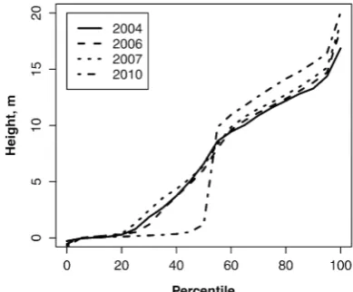
Fig. 6 illustrates multitemporal cumulative LiDAR h-distributions for a 400-m2 area near plot A. The understory trees were cleared in 2009, which shows in the h-distribution of 2010.
Fig. 6. Cumulative LiDAR h-distributions near plot A in an area that was cleared from dense understory in 2009.. The area-based LiDAR metrics were analyzed using univariate regression. The proportion of ground returns over all understory returns was a strong predictor of the density of understory. The R2 values were highest, when Pgnd was contrasted with over 1-m tall trees. The negative correlation was very low, when the density of all understory trees (h > 0.3 m) was contrasted with Pgnd. The correlation thus failed for short trees. The intensity features had mostly positive correlation with density. The positive correlation of intensity and density is explained by the increasing density of overlapping crowns. The h-distribution density metrics showed also strong positive correlation with density. In the sparse data of 2008, the correlations were generally lower than in the dense data sets. The mean h was explained best by h-distribution deciles. The dependencies were not always linear. The estimation of the propor-tion of broadleaved trees showed inconsistent results as the dependencies between intensity deciles and the proportion differed between plots. This could be due to differences in the understory trees as the same correlation structure was observed in all LiDAR data sets. This example confirms that the determination of species proportions can be very challenging in area-based estimation using intensity metrics.
5. DISCUSSION
5.1 Confines of the study
The experiment comprised of carefully measured field reference data and several LiDAR data sets, but the representativeness of the two plots is very limited, as they cover very little of the variation found in two-layer pine stands in Finland. The experiment was best suited for the analysis of transmission losses and pulse-target interaction
5.2 Mapping of the understory trees in the field to the coordinate system of the LiDAR
We presented a new method by which it was possible to map and measure about 40 understory trees per hour directly into the coordinate system of the LiDAR under poor visibility.
5.3 Echo-triggering of the sensors and geometry of the LiDAR data in the understory
The pulse penetration maps showed that pulses that are free from transmission losses reach the understory through the large openings in the canopy. Multi-return pulses had a particular spatial pattern, as they are concentrated in areas near the edges of crown project-ions. Very few pulses reached the ground if the pulse path had tra-versed the crown near the stem of an overstory tree. Our results imply that the echo-triggering probabilities in the understory trees may be dependent on the species. This complicates estimation of species proportions and may skew the density and h estimates in stands comprising of several species. As could be expected, the overstory affected the echo-triggering probabilities and geometry in the different echo classes. These findings are not original, but show that our experiment had high geometric accuracy. There were diffe-rences between sensors in their ability to measure the shortest trees, which was due to differences in the echo-triggering mechanisms and the blind zone that follows (and precedes) an echo. This clearly shows that the radiometry and geometry in LiDAR data can not be looked at independently. If an echo can be triggered in the under-story depends both on the signal available and the target size being intersected. The near-ground h-distributions can vary considerably between sensors, as was shown in our data. Even the gain control in the receiver was shown to affect echo-triggering in the understory. 5.4 Intensity data in the understory tree-layer
Species-specific differences in intensity were very marginal and first-return data is by far most useful. High noise prevailed in the second and third-return data and it was reduced with the ran-ge/AGC-correction and transmission-loss models. The compensat-ion of transmisscompensat-ion losses is an ill-posed task in LiDAR data, and our models attempted it by considering the intensity observations of previous returns and the geometry of the pulse path. This was only possible since the overstory was rather homogenous on both plots. The geometric information proved useful. Different methods for computing the losses due to geometry were tried, but they all provided similar best-case results. We tested a Beer’s law approach and used simple, functional approximations of foliage density dist-ribution. It is evident that the scatterers in pine crowns are clumped and the assumption of a turbid medium does not hold. We could even show that first-return data in the understory is subject to losses by weak interactions that do not trigger echoes in the overstory. The CVs of intensity in the understory increased with scanning alti-tude, and there were differences between the two sensors, which, in first-return data were due to the differences in echo triggering. In-tensity-based classification of ground and dominant understory spe-cies was improved, when transmission losses were corrected in second and third-return data for both sensors. However, the accura-cy remained low. It seems that the first-, second- and third-return intensity observations from the understory differ such that they can-not be normalized to a single intensity variable. Single returns are generated by dense and/or reflective scatterers and show higher mean intensity and lower CV than other returns. First returns can vary from noise-level to strong reflections. A second or third return occurs in a pulse that has been subject to transmission losses, and the scatterers have to be reflective and/or large with respect to the illuminated area, to trigger an echo. This means that the echoes rep-resent different scatterer populations. At the pulse-level, we could show that intensity was dependent on factors such as the local den-sity of the understory, horizontal distance from the stem of the in-tersected understory tree, and the length of the pulse path in the understory tree.
5.5 Area-based estimation of forestry variables in the understory tree
Our results are partly in line with those in Maltamo et al. (2005). However, their LiDAR h-distribution metrics included observations
from the dominant trees, while our LiDAR metrics were confined explicitly to the understory, and indirect correlations of via the overstory were not employed. Our results showed that h-distribut-ion metrics could be used for the estimath-distribut-ion of the density of the understory, when restricting to trees with h > 1 m. Intensity metrics were dependent on the local density of the understory, but showed inconsistent dependencies with the proportion of broadleaved trees. The results on intensity are disappointing, because species discrimi-nation is so important.
5.6 Conclusions
Intensity normalization in discrete-return data for the transmission losses occurring in the overstory was feasible to some degree, but did not significantly improve the usability of intensity data in multi-return pulses. Non-seen losses that are due to weak intersections were shown decrease the intensities up to 10% in the understory. Full-waveform LiDAR data is fundamentally different, and the compensation of the losses could be feasible in such data and we propose research in that topic. LiDAR h-distribution metrics have potential in area-based detection and assessment of the understory. However, in our case the intensity data seems too noisy for reliable species discrimination, which is a serious deficiency considering practical applications in forest inventory.
REFERENCES
Hill, R. A., Broughton, R. K., 2009. Mapping understory from leaf-on and leaf-off airborne LiDAR data of deciduous woodland. ISPRS JPRS, 64, pp. 223−233.
Korpela, I., 2008. Mapping of understory lichens with airborne dis-crete-return LiDAR data. RSE, 112, pp. 3891−3897.
Korpela, I. , Tuomola, T., Tokola, T., Dahlin, B., 2008. Appraisal of seedling stand vegetation with airborne imagery and discrete-re-turn LiDAR – an exploratory analysis. Silva F, 42, pp. 753−772. Korpela, I., Ørka, H. O., Heikkinen, V., Tokola, T., Hyyppä, J., 2010. Range- and AGC normalization of LIDAR intensity data for vegetation classification. ISPRS JPRS, 65, pp. 369−379.
Maltamo, M., Packalén, P., Yu, X., Eerikäinen, K., Hyyppä, J. Pitkänen, J., 2005. Identifying and quantifying structural character-istics of heterogeneous boreal forests using laser scanner data. For. Ecol. Manag., 216, pp. 41-50.
Martinuzzi, S., Vierling, L.A., Gould, W.A., Evans, J., Falkowski, M., Hudak, A. Vierling, K.T., 2009. Mapping snags and understo-ry shrubs for a LiDAR-based assessment of wildlife habitat suitabi-lity. RSE 113, pp. 2533–2546
Morsdorf, F., Mårell, A., Koetz, B., Cassagne, N., et al. Pimont, F., Rigolot, E., Allgöwer, B., 2010. Discrimination of vegetation strata in a multi-layered Mediterranean forest ecosystem using height and intensity information derived from airborne laser scanning. RSE, 114, pp. 1403–1415.
Næsset, E., 2004. Practical Large-scale forest stand inventory using a small-footprint airborne scanning laser. Scand. J. For. Res., 19, pp. 164–179.
Ørka, H.O., Næsset, E., Bollandsås, O.M. 2009. Classifying species of individual trees by intensity and structure features derived from airborne laser scanner data. RSE, 113, pp. 1163–1174.
Peltoniemi, J., Kaasalainen, S., Näränen, J., Rautiainen, M., Sten-berg, P., Smolander, H., et al. 2005. BRDF measurement of under-story vegetation in pine forests: dwarf shrubs, lichen, and moss. RSE, 94, pp. 343−354.