A NEW FEATURE DESCRIPTOR FOR LIDAR IMAGE MATCHING
M. Jayendra-Lakshmana,∗and V. Devarajana
a
Dept. of Electrical Engineering, University of Texas at Arlington Arlington, Texas, USA [email protected], [email protected]
KEY WORDS:LiDAR, Computer Vision, Point Matching, Feature Descriptor
ABSTRACT:
LIght Detection And Ranging (LiDAR) data is available in a point cloud corresponding to long overlapping strips on the ground. The percentage of overlap in these LiDAR strips varies between 10 and 30. The strips are unregistered with respect to each other. Any further interpretation or study of the whole area requires registration of these strips with respect to each other. This process is called strip-adjustment. Traditionally, LiDAR point clouds are matched and strip-adjusted using techniques based on iterative closest point (ICP) or modifications of the same, which as the name suggests, runs over multiple iterations. Iterative algorithms, however, are time consuming and this paper offers a solution to the problem. In this paper, point correspondences are found on overlapping strips so that they can be registered with each other. We introduce a new method for point matching on LiDAR data. Our algorithm combines the power of LiDAR elevation data with a keypoint detector and descriptor that is based on the Scale Invariant Feature Transform (SIFT) method. The keypoint detector finds interesting keypoints in the LiDAR intensity image from the SIFT keypoints; a unique signature of each keypoint is then obtained by examining a patch surrounding that point in the elevation image. Histograms of subdivisions of the patch are set as the keypoint descriptor. Once all the keypoints and descriptors are obtained for two overlapping patches, correspondences are found using the nearest neighbor distance ratio method.
1 INTRODUCTION
1.1 LiDAR Introduction
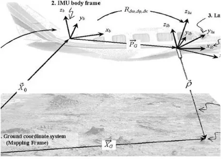
A LiDAR system consists of a laser ranging and scanning unit together with a position and orientation system. There are two components to this system: inertial measurement unit (IMU) and the integrated differential Global Positioning System (GPS). The laser ranging unit measures distances from the sensor to the mapped surface, while the onboard GPS/IMU component provides the po-sition and orientation of the platform. LiDAR data collection is carried out in a strip-wise fashion, and the ground coordinates of LiDAR points are derived through a vector summation process. The LiDAR system setup is shown in Figure 1. (Habib et al., 2010)
Figure 1: LiDAR data acquisition
The LiDAR system mathematical model is given by the equation:
~
XG=X~0+Ryaw,pitch,rollP~G+Ryaw,pitch,rollR∆ω,∆φ,∆χRα,β
0 0
−ρ
(1)
where,X~Ggives the position of the object point on the ground. Proper rotations are applied to the three vectorsX~0,P~Gand~ρ.
~
X0 is the translation between the ground coordinate frame and the IMU body frame.
~
PGis the translation vector between the IMU body frame and the laser unit.
~
ρis the translation between the object point and the laser unit.
Rα,βis the rotation matrix relating the laser unit and laser beam coordinate systems withαandβbeing the mirror scan angles.
R∆ω,∆φ,∆χis the rotation matrix relating the IMU and laser unit coordinate systems.
andRyaw,pitch,rollis the rotation matrix relating the ground frame-work and IMU coordinate systems.
The surface representation of LiDAR data is available as a point cloud where each point can be described asPx,y,z,i. Herexand
yare the 2D locations on the ground plane andz is the eleva-tion informaeleva-tion above mean sea level; iis the intensity of the reflected light pulse. The value ofz, is a continuous function at the(x, y)points on the ground. However, for practical purposes, we need to use a discrete representation (Shan and Toth, 2009):
Ed
ij=Qp(Sc) =Qp(f(xk, yk)) (2)
Where,Eijd is the discrete surface elevation,
Qpis the quantization function that maps the continuous repre-sentationScto2pdiscrete levels,
andSc=f(xk, yk)andxi,yiare the 2D sampling locations.
1.2 Feature Detector-Descriptor
Image matching is the process of finding common points or com-mon patches in two images and determining if there are simi-lar objects in them. Image matching techniques can be broadly classified into two types: area based methods, and feature based methods (Brown, 1992). Area based methods are template match-ing techniques which aim to match specific patches of a query image with patches of a template image. These methods match patches with a correlation/similarity score and are weak, in that, they need to be adapted in order to cope up with scale or rotation changes. Making them perspective invariant needs further adap-tation and can be very costly from a compuadap-tational load point of view. When a simple template matching fails, matching is at-tempted in the Fourier domain or by mutual information content in the images. These methods are brute-force in nature.
This paper will focus its attention on feature based techniques.
Feature based techniques are the ones that use distinctiveness in the images in order to establish correspondences. They make use of the mutual-relationship among pixels within an interest-ing neighborhood unlike area based methods which require ex-amination of normalized cross-correlation scores of every possi-ble overlapping patch. Such a treatment is particularly impor-tant, when there are changes in viewpoints or viewing condi-tions. Most feature based techniques make use of local feature descriptors of interest points to capture their uniqueness. The task of finding interesting points is called interest point detec-tion. Some techniques blur the same image at different scales and levels of blur using a Gaussian function; the keypoints are the points that remain as maximas at different levels of blur for each scale (Lowe, 2004). These scales are used in sampling of points in the neighborhood to form unique, invariant descriptors. Feature based techniques aim to reduce the dimensionality of rep-resented data without compromising the uniqueness of the inter-esting points. In this vein, this paper introduces a technique for matching LiDAR images based on local feature descriptors. The remainder of this section provides brief descriptions of the broad subtasks in the workflow of feature based matching:
1. INTEREST POINT DETECTION: The first step is the process of finding the locations of interest points, linear struc-tures, curves or even complex structures that may or may not have perceivable order to them. The interest points could be edge pixels, corner points or local maxima/minima of image intensity. Linear structures could be lines or shapes that con-tain lines in them. There are also other non-linear curves that have a structure to them such as splines, which are used in many interpolation techniques to fill in missing information. The more complex structures could be manmade objects, or naturally occurring objects in the image.
2. LOCAL FEATURE DESCRIPTOR: The second step is to create a local descriptor of the immediate neighborhood of the feature location to make it unique/different from the other features in the images. This is accomplished with enough precaution to avoid mismatches or misidentifications among interest points, while assuring a high degree of simi-larity to the same feature in another view of the image.
One image of the same scene and objects can be very dif-ferent from another image of the same content based on many factors. They can range from distortion caused by errors in the acquisition process like radial distortion etc., difference in the modalities of the image capture, occlusion of certain objects in the scene, illumination changes due
to viewing conditions and most common of all, change in viewing point. The change in viewpoint can result in per-spective variation or affine transformation including zoom-ing or pannzoom-ing, which may lead to effects that change shapes of objects or cause partial/full occlusion of certain objects. Therefore, it is not sufficient to have features that are salient; these features must be repeatable in many views of a scene and must be robust if not invariant to the aforementioned changes. This is the principal area of research of this paper.
3. POINT MATCHING: After local features are defined, a point-matching scheme needs to be applied to find similar points in two images by means of analyzing the descrip-tors. Matches are found by evaluating a similarity mea-sure or distance meamea-sure. The actual implementation of such a scheme requires evaluating a distance or similarity score of every interest point in one image against every in-terest point in the other image. Bad matches are eliminated and good matches are picked after comparing the best match score against other match scores for each set of correspon-dences. Some of the match steps are accomplished by a) using thresholds to select good matches; b) evaluating the nearest neighbor, which is the best match score for a point in the template image for a point in the query image; or c) evaluating the nearest neighbor distance ratio. The nearest-neighbor distance ratio is an extension of the nearest neigh-bor technique that uses a threshold for the ratio of the scores of the second nearest neighbor to the nearest neighbor.
4. IMAGE TRANSFORMATION: This is the final step of the workflow which finds the transformation of the query image to the template image. The transformation is calcu-lated with an iterative technique or by voting for the best transformations as in the Hough transform used by Duda and Hart (Duda and Hart, 1972). After finding the trans-formation, the image is transformed and re-sampled to be registered with template image.
In this paper, we are going to explore the first three subtasks in image matching.
2 RELATED WORK
Image matching can be accomplished by area based and feature based methods. Area based methods have been used with adap-tion to scale and rotaadap-tion since the 1970s (Anuta, 1970). Zhao (Zhao et al., 2006), adapted the normalized cross-correlation tech-nique for large camera motions within images.
Area based methods match each patch of a predefined size in the image with every patch of the same size in the template image, it is very time consuming. Thus, this paper focuses its attention on feature based techniques and the remainder of the section elabo-rates on the prior work on the same field.
Feature extraction in image processing can be used for various applications. Some of them are wide baseline stereo matching, 3D reconstruction, image mosaicking, texture recognition, im-age retrieval, object classification, object recognition to name a few. In the field of local feature descriptors, much work has been done since the advent of the Harris corner detector (Harris and Stephens, 1988), which is a very strong interest point detector. Corners are relatively invariant to changes in viewpoints with a high degree of robustness.
1. (Mikolajczyk and Schmid, 2001) introduced a new scale invariant technique by adapting interest points to changes in scale (Dufournaud et al., 2000). They used the Harris corner detector and selected points where the Laplacian at-tained maximum over scales. Their local feature descrip-tors were Gaussian derivatives computed at the characteris-tic scale and they achieved invariance to rotation by steering the derivatives in the direction of the gradient at the interest point. The technique introduced here is useful due to the fact that the descriptor can be scale-adapted for a stronger invariance, a result that contributes to this paper.
2. (Lowe, 2004) introduced the Scale Invariant Feature Trans-form (SIFT), a technique that implemented a difference-of-Gaussian function on multiple scales of the same image at every pixel location as a key point detector. This technique approximated the Laplacian of Gaussian very well and in a more computationally cost effective manner (Lindeberg, 1994). Further, the algorithm found exact location and scale by using a Taylor expansion of the scale space function (Brown and Lowe, 2002). The dominant orientation was used to steer the descriptor to make it rotationally invariant. Finally, the local descriptors were obtained by examining a 16×16 patch about the interest point that had been weighted by a Gaussian window. An 8-bin histogram of gradient orienta-tions for each 4×4 patch (there are 16 in total) was obtained and the data was concatenated to from a descriptor that has 128 dimensions. SIFT forms the basis of the descriptor in-troduced in this paper. The descriptor is shown in Figure 2 (Lowe, 2004)
Figure 2: SIFT descriptor
3. (Mikolajczyk and Schmid, 2005), introduced Gradient Lo-cation and Orientation Histogram (GLOH), an extension of the SIFT descriptor designed to increase its robustness and distinctiveness. The SIFT descriptor was computed for a log-polar location grid with three bins in radial direction with the radius set to 6, 11, and 15 and 8 in angular di-rection, which resulted in 17 location bins. They compared the performance of GLOH to SIFT, PCA-SIFT (Ke and Suk-thankar, 2004) and other previously-introduced techniques. Their inference was that SIFT and GLOH predominantly performed better than other descriptors detector for vari-ous matching techniques, viewpoint changes, scale-changes, blur, JPEG compression and illumination changes. GLOH is an interesting idea which might be explored in the future work of this paper.
4. (Zitova and Flusser, 2003) reviewed existing methods of im-age registration of multimodal imim-ages and imim-ages acquired from various viewpoints. The methods included area-based techniques correlation based, Fourier methods and mutual information; and feature based techniques methods involv-ing spatial relations, methods based on descriptors, relax-ation methods and pyramids and wavelets. It also provided surveys of the transform model estimation for linear and non-linear cases.
These are techniques that are used traditionally on camera (opti-cal) images. For LiDAR point cloud data, there have been some feature descriptors that have been developed in literature. They are listed below:
1. (Li and Olson, 2010) introduced a general-purpose feature detector based on image processing techniques. It employs Kanade-Tomasi corner detector (Shi and Tomasi, 1994) to detect key points and the angle descriptor contains four an-gles, the first three are the angles formed by the extracted corner and the three point sets that are d, 2d and 3d meters away from the extracted corner, and the fourth angle is the heading of the corner. The three point sets are generated by finding the intersection of circles of radii d, 2d and 3d me-ters. The line segments are then formed by joining actual LiDAR points. Figure 3 (Li and Olson, 2010) shows an illustration of the formation of the descriptor.
Figure 3: Li & Olson descriptor
2. Moment gridis a descriptor introduced in (Bosse and Zlot, 2009). The key point detector is the same as SIFT, while the descriptor is formed by evaluating eight descriptor elements that are computed from the weighted moments of oriented points(xi, yi, θi)for a total of 13 grids with the detected key point in the center. Thus the total size of the descriptor is 13×8=104. These grids could be a 2×2 or a 3×3 region as shown in Figure 4 (Bosse and Zlot, 2009).
Figure 4: Moment grid descriptor
3 ELEVATION BASED FEATURE DESCRIPTOR
A key point detector and feature descriptor have been proposed and tested which match corresponding points in two or more Li-DAR strips. The novelty of the descriptor lies in the fact that no technique exists in the literature that makes use of LiDAR inten-sity and elevation simultaneously; and very few techniques exist that attempt to match and register data using a local feature de-scriptor. The following describe the steps of our approach.
3.1 INTERPOLATION
The LiDAR point cloud data was interpolated by the inverse dis-tance weighted (IDW) method (Shepard, 1968). This method, as the name suggests, interpolates the elevation and intensity of a point by weighted averaging of nearby LiDAR points.
3.2 KEYPOINT DETECTION
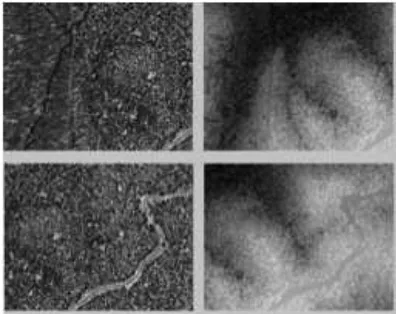
(Lindeberg, 1998) showed that Gaussian blurring of an image provides a scale-space for the image. The Laplacian of the image provides excellent key points that are invariant to viewing condi-tions (Mikolajczyk and Schmid, 2004), (Lowe, 2004). It is possi-ble to obtain an approximation of the Laplacian by performing the difference of Gaussian. These results were applied in the imple-mentation of SIFT. In this algorithm, the interest point detection uses the same detector to single out salient points in the image. The SIFT detector is applied on the intensity image. The rationale is that sharp changes in elevation don’t necessarily result in sharp changes in the image representation of the same area. However, the LiDAR intensity image could contain corner-like features due to its proximity to optical images. Figure 5 shows experimental results after interpolation on an image created by inverse distance weighted interpolation on LiDAR data from Yosemite National Park. This data was obtained from open-topography. The data, which contains little more than 400000 points, is split up into two overlapping datasets to create two 450×578 images. The in-terpolation technique, as mentioned in the background section, finds all points that lie within a specified distance of each pixel location and interpolates the pixel’s intensity and elevation values based on inverse weights. Figure 5 shows the intensity images of overlapping data on the left and the elevation images on the right. It is easier to obtain corner points on the intensity image, given the flat nature of elevation that can be expected in many elevation maps. Figure 6 shows the keypoints obtained.
Figure 5: LiDAR intensity and elevation images
3.3 KEYPOINT DESCRIPTOR
The key point descriptor evaluates the histogram of elevations in the neighborhood of the detected key point location. Histograms
Figure 6: Keypoints extracted with SIFT detector
of local sub-patch make it possible to compact the information from the sub-patch into a smaller dimensionality. This facilitates matching more quickly and eliminates missed matches caused by interpolation errors (compacting the data into a histogram reduces the exactness required for a match). Also, it is a well-understood technique employed in SIFT (Lowe, 2004), GLOH (Mikolajczyk and Schmid, 2005) and PCA-SIFT (Ke and Sukthankar, 2004).
Elevations of points on earth are invariant to changes in viewing conditions or viewpoints. Thus, gradients do not have to be used as invariant parameters of the pixel locations as is done in SIFT. Elevation points on a 16×16 grid about the key point were ex-tracted. The advantage of using the SIFT based key point detec-tor comes into play here. The SIFT detecdetec-tor comes with a scale for each key point. This enables sampling of points about the key point at the sub-pixel level according to the scale of the key point. This step is important in our algorithm as well, because the best information about the point cannot be obtained without sampling at the prescribed scale.
The reason why a 16×16 grid was chosen for the descriptor is that by having a smaller grid with smaller subpatches, it is difficult to create a unique descriptor. The same experiment was conducted using an 8×8 patch and the number of point matches reduced to less than half the matches from a 16×16 patch but it took more than half as much time. Also, the experiment was repeated for a 32×32 patch about the key point. This resulted in just 3% more matches. The 16×16 patch was finalized as the patch size for the descriptor based on the above results.
The following steps were undertaken to evaluate the invariant keypoint descriptor:
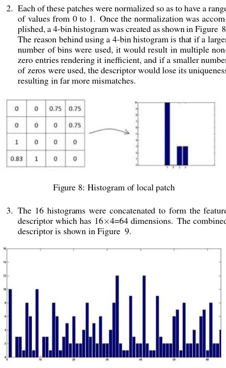
1. For every key point location detected by the detector algo-rithm, in the corresponding elevation image, a 16×16 patch about the key point location was extracted. This patch was subdivided into 16 patches of size 4×4 each. These are ex-tracted starting at the top left, going all the way to the bottom right. The process is shown in Figure 7.
2. Each of these patches were normalized so as to have a range of values from 0 to 1. Once the normalization was accom-plished, a 4-bin histogram was created as shown in Figure 8. The reason behind using a 4-bin histogram is that if a larger number of bins were used, it would result in multiple non-zero entries rendering it inefficient, and if a smaller number of zeros were used, the descriptor would lose its uniqueness resulting in far more mismatches.
Figure 8: Histogram of local patch
3. The 16 histograms were concatenated to form the feature descriptor which has 16×4=64 dimensions. The combined descriptor is shown in Figure 9.
Figure 9: Final descriptor after concatenation
Given the probabilistic nature of the problem, the best patch size and the number of bins needed for the histogram in each patch, have been experimentally determined. Since the process is highly non-linear, a combination of local statistics (histogram) and adap-tive parameters is desired (number of bins & number of patches) for achieving the goals.
3.4 POINT MATCHING
The point-matching algorithm first looks for the nearest neighbor for points in either image. After this, if the ratio of the second nearest matching distance to the nearest neighbor is examined. A match is eliminated if the ratio is below a preset threshold. This is the nearest neighbor distance ratio technique (Lowe, 2004). The following is done to finding correspondences: Let us call the two images asI1and I2. Firstly, for each key point inI1, the squared distance is measured for each key point inI2. The best match for a key point inI1 is found inI2. False matches are eliminated by examining the 2nd best distance and, disregarding the correspondence if the ratio of the 2nd distance to the matching distance is less than 2.
4 RESULTS
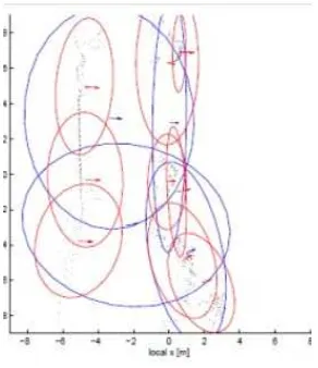
Shown in Figure 10 are the matching intensity and elevation im-age points based on this algorithm. There were 284 matches for these images.
Figure 10: Matches for descriptor based only on elevation data
A similar experiment was done on intensity data. A descriptor was created from the patch in the intensity data within the neigh-borhood of the detected keypoints. This descriptor resulted in 334 matches (17% more than descriptor based only on elevation data. Matches shown in Figure 11).
Figure 11: Matches for descriptor based only on intensity data
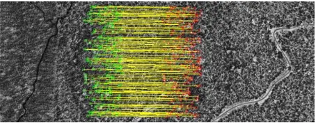
The fact that the intensity based descriptor gave more matches than the descriptor based only on elevation data prompted us to combine both elevation and intensity data. The elevation and Li-DAR intensity data are perfectly co-registered. Thus, we obtained a new descriptor by concatenating the histograms obtained from the local elevation data and the local intensity data. The resulting descriptor is 2×16×4=128 dimensions long. This descriptor re-sulted in 381 matches (34% more than descriptor based only on elevation data. Matches shown in Figure 12).
Figure 12: Matches for combined elevation-intensity descriptor
4.1 COMPARISON WITH SIFT
A direct comparison was made by running the SIFT algorithm on the same images. By running the SIFT algorithm on intensity data alone, the number of matches obtained was 385 (35% more than the descriptor based only on elevation data). The matches are shown in Figure 13. These results are similar to the com-bined keypoint descriptor introduced in this paper; the advantage of the descriptor we introduced is that it is less computationally intensive than SIFT due to the fact that SIFT does an additional computation of obtaining gradient orientations and magnitudes.
matches obtained from the combined elevation-intensity descrip-tor. The reason for this is because the keypoint detection algo-rithm run for the descriptors introduced in this paper is the SIFT detector. In future, alternative keypoint detection schemes will be explored from the LiDAR elevation and intensity data. We expect this will result in keypoints that are different from SIFT keypoints. This approach will likely showcase the combined el-evation and intensity data approach to point matching even more than in this paper since SIFT is typically used on optical images alone.
Figure 13: Matches for SIFT using intensity data
5 CONCLUSION
In this paper we have introduced a feature descriptor for LiDAR intensity and elevation data based on the Scale Invariant Feature Transform. The novelty of the method lies in the fact that both the elevations and intensities are used, like an image to form a descriptor and match points directly on the interpolated raster data. The combination of the feature descriptor and point match-ing technique can be used to obtain a transformation to register overlapping LiDAR point cloud data.
Future work includes exploration of alternative interpolation tech-niques, namely, Sparsity coding based interpolations, alternative keypoint detection techniques that could work in the absence of LiDAR intensity data and feature descriptors based on log-polar grids and ones with reduced dimensionality. A detailed compar-ison with existing techniques in Image processing and in LiDAR point matching needs to be done in the future.
REFERENCES
Anuta, P. E., 1970. Spatial registration of multispectral and multi-temporal digital imagery using fast fourier transform techniques. Geoscience Electronics, IEEE Transactions on 8(4), pp. 353–368.
Bosse, M. and Zlot, R., 2009. Keypoint design and evaluation for place recognition in 2d lidar maps. Robotics and Autonomous Systems 57(12), pp. 1211–1224.
Brown, L. G., 1992. A survey of image registration techniques. ACM computing surveys (CSUR) 24(4), pp. 325–376.
Brown, M. and Lowe, D. G., 2002. Invariant features from inter-est point groups. In: British Machine Vision Conference, Cardiff, Wales, Vol. 21number 2, pp. 656–665.
Duda, R. O. and Hart, P. E., 1972. Use of the hough transforma-tion to detect lines and curves in pictures. Communicatransforma-tions of the ACM 15(1), pp. 11–15.
Dufournaud, Y., Schmid, C. and Horaud, R., 2000. Matching im-ages with different resolutions. In: Computer Vision and Pattern Recognition, 2000. Proceedings. IEEE Conference on, Vol. 1, IEEE, pp. 612–618.
Habib, A., Kersting, A. P., Bang, K. I. and Lee, D.-C., 2010. Al-ternative methodologies for the internal quality control of parallel lidar strips. Geoscience and Remote Sensing, IEEE Transactions on 48(1), pp. 221–236.
Harris, C. and Stephens, M., 1988. A combined corner and edge detector. In: Alvey vision conference, Vol. 15, Manchester, UK, p. 50.
Ke, Y. and Sukthankar, R., 2004. Pca-sift: A more distinctive rep-resentation for local image descriptors. In: Computer Vision and Pattern Recognition, 2004. CVPR 2004. Proceedings of the 2004 IEEE Computer Society Conference on, Vol. 2, IEEE, pp. II–506.
Li, Y. and Olson, E. B., 2010. A general purpose feature extractor for light detection and ranging data. Sensors 10(11), pp. 10356– 10375.
Lindeberg, T., 1994. Scale-space theory: A basic tool for ana-lyzing structures at different scales. Journal of applied statistics 21(1-2), pp. 225–270.
Lindeberg, T., 1998. Feature detection with automatic scale se-lection. International journal of computer vision 30(2), pp. 79– 116.
Lowe, D. G., 2004. Distinctive image features from scale-invariant keypoints. International journal of computer vision 60(2), pp. 91–110.
Mikolajczyk, K. and Schmid, C., 2001. Indexing based on scale invariant interest points. In: Computer Vision, 2001. ICCV 2001. Proceedings. Eighth IEEE International Conference on, Vol. 1, IEEE, pp. 525–531.
Mikolajczyk, K. and Schmid, C., 2004. Scale & affine invariant interest point detectors. International journal of computer vision 60(1), pp. 63–86.
Mikolajczyk, K. and Schmid, C., 2005. A performance evaluation of local descriptors. Pattern Analysis and Machine Intelligence, IEEE Transactions on 27(10), pp. 1615–1630.
Shan, J. and Toth, C. K., 2009. Topographic laser ranging and scanning: principles and processing. CRC Press.
Shepard, D., 1968. A two-dimensional interpolation function for irregularly-spaced data. In: Proceedings of the 1968 23rd ACM national conference, ACM, pp. 517–524.
Shi, J. and Tomasi, C., 1994. Good features to track. In: Computer Vision and Pattern Recognition, 1994. Proceedings CVPR’94., 1994 IEEE Computer Society Conference on, IEEE, pp. 593–600.
Zhao, F., Huang, Q. and Gao, W., 2006. Image matching by normalized cross-correlation. In: Acoustics, Speech and Signal Processing, 2006. ICASSP 2006 Proceedings. 2006 IEEE Inter-national Conference on, Vol. 2, IEEE, pp. II–II.