SPATIOTEMPORAL DOMAIN DECOMPOSITION FOR MASSIVE
PARALLEL COMPUTATION OF SPACE-TIME KERNEL DENSITY
Alexander Hohl a,b*, Eric M. Delmelle a,b, Wenwu Tang a,b a
Department of Geography and Earth Sciences, University of North Carolina at Charlotte, 9201 University City Blvd, Charlotte, NC, 28223, USA
b
Center for Applied Geographic Information Science, University of North Carolina at Charlotte, 9201 University City Blvd, Charlotte, NC, 28223, USA
Email: (ahohl, Eric.Delmelle, WenwuTang)@uncc.edu
KEY WORDS: Domain Decomposition, Parallel Computing, Space-Time Analysis, Octtree, Kernel Density Estimation
ABSTRACT:
Accelerated processing capabilities are deemed critical when conducting analysis on spatiotemporal datasets of increasing size, diversity and availability. High-performance parallel computing offers the capacity to solve computationally demanding problems in a limited timeframe, but likewise poses the challenge of preventing processing inefficiency due to workload imbalance between computing resources. Therefore, when designing new algorithms capable of implementing parallel strategies, careful spatiotemporal domain decomposition is necessary to account for heterogeneity in the data. In this study, we perform octtree-based adaptive decomposition of the spatiotemporal domain for parallel computation of space-time kernel density. In order to avoid edge effects near subdomain boundaries, we establish spatiotemporal buffers to include adjacent data-points that are within the spatial and temporal kernel bandwidths. Then, we quantify computational intensity of each subdomain to balance workloads among processors. We illustrate the benefits of our methodology using a space-time epidemiological dataset of Dengue fever, an infectious vector-borne disease that poses a severe threat to communities in tropical climates. Our parallel implementation of kernel density reaches substantial speedup compared to sequential processing, and achieves high levels of workload balance among processors due to great accuracy in quantifying computational intensity. Our approach is portable of other space-time analytical tests.
* Corresponding author
1. INTRODUCTION
Performance and computational complexity have hampered scientific investigations and decision making, which is especially dreadful in such arenas as spatial epidemiology, where inefficient computation may impact the timely detection of infectious disease clusters. First, the amount of data collected increases by orders of magnitude with the advancement of, for example, sensor systems and automated geocoding abilities which allows for increasingly realistic representations of spatial processes. Second, many geographic models are computationally intensive because of search strategies that explode as a function of problem size due to multiple levels of nested iterations. As more scientists discover new analysis paradigms that are data-intensive, increasing computational requirements raise the need for high performance computing (Armstrong, 2000). Implementing parallel strategies has the potential to meet the demand for increased processing power (Wilkinson and Allen, 1999). Therefore, we need to design, modify, or extend new geographic algorithms, taking advantage of parallel computing structures, and allowing us to mitigate performance and computational complexity issues for better support of scientific discovery and decision making.
Parallel computing allows for time-efficient processing of massive datasets, but to prevent workload imbalance and therefore, processing inefficiency, their spatiotemporal characteristics have to be accounted for (Wang and Armstrong,
2003). The general strategy is to decompose the spatiotemporal domain of a dataset, distribute the resulting subdomains to multiple computing resources for concurrent processing, and finally collect and reassemble the results (Wilkinson and Allen, 1999). While random or uniform data can be decomposed by non-adaptive column-wise division or regular tessellations, doing so for clustered datasets results in heterogeneous subdomains in terms of computational intensity as they contain uneven quantities of data (Ding and Densham, 1996). Therefore, subdomains of similar or equal computational intensity are conducive for load balancing and for flexibility in distributing jobs to processor queues. Consequently, adaptive and recursive domain decomposition methods, such as quadtrees, have been widely used for mitigating workload imbalance for 2D models within the geographical realm (Turton, 2003; Wang and Armstrong, 2003).
However, the recent trend within geographic research to include time as a third dimension, together with the advent of big spatiotemporal data, further increase the importance of strategies to handle complex computations on massive datasets (Kwan and Neutens, 2014). Therefore, we need to revisit the domain decomposition strategy, and complement it with the ability to handle real-world massive spatiotemporal data, in order to meet the recently emerging requirements of scientific investigation and decision making. To our knowledge, the recursive decomposition of massive spatiotemporal datasets for ISPRS Annals of the Photogrammetry, Remote Sensing and Spatial Information Sciences, Volume II-4/W2, 2015
parallel processing has been insufficiently addressed in the literature so far.
In this study, we perform octtree-based recursive decomposition of the space-time domain for parallel computation of kernel density on a spatiotemporally explicit dataset. In order to handle edge effects near subdomain boundaries, we implement spatiotemporal buffers to include adjacent data points that are within the spatial and temporal bandwidths, but outside the subdomain under consideration. To balance workloads among processors, we quantify the computational intensity of each subdomain for subsequent distribution among processor queues, equalizing the cumulative computational intensity among them. We illustrate the benefits of our methodology using a space-time epidemiological dataset of Dengue fever, an infectious vector-borne disease. We report metrics and results that illustrate gain in performance and workload balance of our parallel implementation. Our work contributes to the advancement of parallel strategies for complex computations associated with the analysis of massive spatiotemporal datasets and their inherent heterogeneity.
2. DATA
Dengue fever is vector-borne disease which is transmitted between humans by mosquitoes of the genus Aedes, posing severe problems to communities and health care providers (Delmelle et al., 2014). We used geocoded cases of Dengue fever in the city of Cali, Colombia during the epidemic of 2010. The data stems from the public health surveillance system and contains 9,555 records, for which coordinates and a timestamp (x, y, t) are provided. The dataset is highly clustered in space and time, as the majority of cases occurred within certain neighborhoods during the first 4-5 months of the year. The Dengue cases were geocoded to the closest street intersection, which guarantees a certain degree of confidentiality. The spatiotemporal cuboid envelope of our study area/period, defined by minimum/maximum values of Dengue cases, spans over 14,286 m in east-west direction, 21,349 m north-south, and over 362 days. traditional kernel density estimation (KDE), and has shown promising results in identifying spatiotemporal patterns of underlying datasets when visualized within the space-time cube framework (Delmelle et al., 2014; Demšar and Virrantaus, 2010; Nakaya and Yano, 2010), where spatiotemporal data are displayed using two spatial (x, y) and a temporal dimension (t). The output is a 3D raster volume where each voxel (volumetric pixel) is assigned a density estimate based on the surrounding point data. The space-time density is estimated by Equation 1 (same notation as Delmelle et al., 2014):
(1)
Density of each voxel s with coordinates (x, y, t) is estimated one-by-one, based on data points (xi, yi, ti) surrounding it. Each point that falls within the neighborhood of the voxel is weighted using a spatial and temporal kernel function, ks and kt, respectively. We used the Epanechnikov kernel (Epanechnikov, 1969) where each data point is weighted according to its proximity in time and space to the voxel s in question (the closer the data point, the higher the weight). The spatial and temporal distances between voxel and data point are given by di and ti respectively. The indicator function I(di < hs; ti < ht) takes on a value of 1 when di and ti are smaller than the spatial (hs) and temporal bandwidth (ht) respectively, otherwise 0. The values of hs and ht are usually identified by a preliminary computation of space-time K-function. For STKDE of the Dengue fever dataset, we set hs and ht to 750 meters and 3 days, respectively, which was determined by Delmelle et al. (2014). We used a spatiotemporal voxel-resolution of 100m * 100m * 1 day within our experimental treatments.
3.2 Spatiotemporal Domain Decomposition
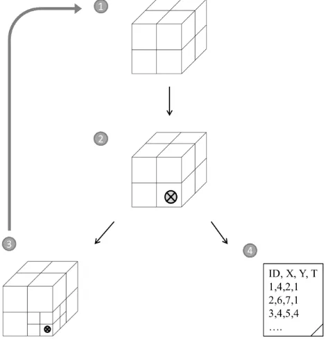
To perform parallel STKDE, we decomposed the Dengue fever dataset for subsequent distribution of the resulting subdomains to processor queues for concurrent processing. We created subdomains of similar computational intensity in order to achieve equal workloads among CPUs. Computational intensity of STKDE mainly depends on 1) the number of data points within the subdomain, 2) the number of voxels, which is given by subdomain size, as voxels are structured within a regularly spaced 3D grid. In order to account for Dengue fever data structure, we used recursive spatiotemporal domain decomposition. Recursion is a method where the solution to a problem depends on solutions to smaller instances of the same problem (Graham, 1994). Most programming languages support recursion by allowing a function to call itself, given that the stopping criterion is not met yet (we use Python 3.3.5). The algorithm starts with defining the bounding box of the dataset, using the minimum and maximum values of each dimension. Step 1 initializes the first level of decomposition (LD1) by dividing each of the three axes into two equal parts (23=8), generating 8 cuboid subdomains (Figure 1). Step 2 iterates through each subdomain and records the number of data points Np and the number of voxels Nv found within. If Np is above a specified threshold Np(max) or if the minimum level of decomposition LD(min) is not reached yet, step 3 will further decompose the subdomain in a recursive manner (reaching LD2), again into 8 subdomains, starting again from step 1. If Np is below the threshold and if LD(min) is reached, step 4 writes the space-time coordinates of data points that are within the current subdomain to a file and the algorithm iterates to the next subdomain. If Np = 0, it moves on without recording any coordinates. Movement across subdomains takes place in Morton order, describing a space-filling z-curve that maps 3D space to one dimension while preserving locality of the data (Bader, 2012). The decomposition produces subdomains that share a set of characteristics: 1) They contain a number of data points Np below a specified threshold Np(max). 2) Their size is restricted by the minimum level of decomposition LD(min), which results in subdomains of smaller or equal size than what LD(min) allows for. The size of the subdomains, and therefore, the number of voxels they contain Nv, decreases with increasing LD in a stepwise manner. The minimum level of decomposition restriction guarantees a certain degree of homogeneity in subdomain size as it prevents the formation of extraordinarily large subdomains that contain only few data points but ISPRS Annals of the Photogrammetry, Remote Sensing and Spatial Information Sciences, Volume II-4/W2, 2015
countless voxels, which proved to be detrimental to workload balance. For our experimental treatments, we set Np = 50 and LD(min) = 4.
Figure 1: Steps of the recursive octtree-based spatiotemporal domain decomposition algorithm.
3.3 Space-Time Buffer Implementation
In order to avoid edge effects in the STKDE which are likely to occur near subdomain boundaries due to the spatial (hs) and temporal bandwidth (ht), we implemented space-time buffers of distance hs and ht around all subdomains. Therefore, if a data point falls outside a subdomain but inside the buffer, the point will still be assigned to that subdomain (and contribute to Np). For sake of simplicity and for easier visualization, Figure 2 provides a conceptual view of the space-time buffer implementation in 2D. As the same concepts apply for 3D, we assume the reader is able to expand her/his mental model of the 2D buffer representation to the spatiotemporal domain (3D). Since the buffers from neighboring subdomains overlap each other, as well as they overlap the neighboring subdomains themselves, data points that fall within these areas are assigned to both subdomains. Therefore, a data point can be assigned to a maximum of 8 subdomains, possibly creating considerable data redundancy, which, however, has not been a problem in our work so far.
3.4 Load Balancing
For each subdomain SDi that resulted from the decomposition, we quantified computational intensity CI as a function of the product of 1) the number of data points Np(SDi) and 2) the number of voxels Nv(SDi) that are contained in the corresponding subdomain (Equation 2).
(2)
To ensure balanced workloads, we distributed the sequence of subdomains (SD1, SD2, …, SDi), resulting from 3D to 1D
mapping by space filling curve, to the processors by equalizing the cumulative CI. Figure 3 provides a conceptual illustration of the approach, where processors receive variable numbers of subdomains but similar workloads. The importance of accurately quantifying CI for our endeavour cannot be stressed enough, as failure of doing so results in failure of balancing workloads. In order to evaluate the accuracy of our quantification of CI, we compared it to execution time T(SDi) for each subdomain. T(SDi) is the actual manifestation of the workload which CI represents, therefore we used linear regression and report R2 to indicate quantification accuracy.
Figure 2: Buffer implementation in 2D with example data points. Each subdomain (solid black lines) is surrounded by a
buffer (dashed grey lines), that therefore, overlap with each other and neighboring subdomains. Example: Point 1 belongs to
SD1 and to the buffer of SD3. Point 2 belongs to SD2, and to the buffers of SD1, SD3, SD4.
Figure 3: Conceptual illustration of load balancing. The cumulative computational intensity CI is evenly distributed
among processors by assigning a varying number of subdomains.
3.5 High-Performance Parallel Computing
After decomposing the dataset and establishing balanced workloads, we performed STKDE in parallel on the VIPER high-performance computing cluster at the University of North Carolina at Charlotte, which has 97 nodes and 984 CPUs that are dual Intel Xeon 2.93 GHz 4-8 core processors with 24-128 GBs of RAM. We varied the number of CPUs in several treatments by varying the number of nodes, choosing one CPU per node. VIPER is a Linux-based cluster that runs TORQUE job scheduling software. We employ the metric of speedup S to evaluate the performance of our parallel STKDE implementation. Speedup is widely used in many parallel applications (Wilkinson and Allen, 1999) and is defined as the ratio between the execution time of the sequential algorithm Ts by that of the parallel algorithm Tp (see Equation 3), which is determined by the slowest processor:
(3)
The closer the speedup is to the number of processors, the better the performance of the parallel algorithm (except in the case of superlinear speedup, when the parallel algorithm uses computing resources more efficiently than the sequential one).
4. RESULTS
4.1 Execution Times and Speedup
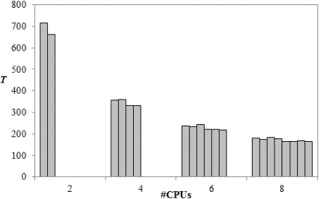
The decomposition resulted in i = 7,177 subdomains, which itself required 62.96 seconds to compute. We applied 5 different treatments, assigning the subdomains to 1, 2, 4, 6, 8 processors for parallel STKDE. With increasing CPUs, execution time T decreased from 1377.54 seconds (sequential time) to 182.90 seconds (parallel time using 8 CPUs) while speedup S increased from 1.93 (2 CPUs) to 7.53 (8 CPUs), both in a non-linear manner (Figure 4). The resulting 3D grid of density values contains 6,302,800 voxels.
Figure 4: Execution time (T) in seconds and Speedup (S) for 1, 2, 4, 6 and 8 CPUs.
4.2 Quantification of Computational Intensity
The relationship between our quantification of computational intensity CI(SDi) and execution time T(SDi) per subdomain, which is the actual manifestation of the workload it represents,
is linear, with an R2 of 0.99. Figure 5 reveals the presence of outliers where CI was either under- or overestimated. Subdomain execution times remain below 1.6 seconds.
Figure 5: Quantification of computational intensity CI versus execution time T(SDi) in seconds (for each subdomain).
4.3 Load Balancing
The accuracy in quantifying CI results in a high level of workload balance, which improves when increasing the number of processors. Figure 6 illustrates execution time T per processor for our 4 parallel experimental treatments. Using 2 processors, the gap between fastest and slowest processor is 53.67 seconds. This gap decreases to 19.19 seconds when using 8 processors.
Figure 6: Load balancing, execution time (T) per processor in seconds.
5. DISCUSSION AND CONCLUSIONS
The reduction of execution time when increasing the number of processors suggests that our approach of spatiotemporal domain decomposition for parallel STKDE was effective. The use of recursive octree decomposition mitigated the problem of workload imbalance between processors and therefore, successfully handled heterogeneity in spatiotemporal data. The quantification of computational intensity is accurate enough to ISPRS Annals of the Photogrammetry, Remote Sensing and Spatial Information Sciences, Volume II-4/W2, 2015
allow for balanced workloads. Our implementation of space-time buffers prevented edge effects in the resulting 3D grid of space-time kernel density values of Dengue fever cases during the 2010 epidemic in Cali, Colombia.
Improvements of our approach will focus on eliminating outliers in computational intensity (Figure 5), which we suspect are caused by the spatiotemporal structure of data points within the subdomain. However, the potential of the outliers to create workload imbalance is limited, as they make up a small fraction of the entire dataset (0.1%) and none of their execution times exceeded 1 second. To date, decomposition time has not been an issue yet, but it might become as we tackle bigger datasets. In addition, as the level of recursion supported by the programming environment may be limited, we anticipate an impediment of our approach when attempting fine-grain decomposition of big datasets.
Our future research will be directed towards testing robustness of the decomposition algorithm by performing sensitivity analysis through parameter variation and subsequent analysis of the effect on execution time and workload balance. Parameters of interest are the maximum number of data points per subdomain, the spatiotemporal resolution of the resulting kernel density grid, the size of the space-time buffers, and the size of the input dataset. We recognize that, due to its limited size, the
Dengue fever dataset cannot be described as “massive”, but it is
rich in hidden patterns and we see it as a useful first step for the development of our parallel approach before moving on to bigger datasets. However, since performing STKDE is computationally challenging, as is illustrated by the large number of voxels in the resulting density grid, we consider it a
“massive” computation.
Our decomposition strategy can be applied to other space-time analysis methods as well. This work contributes to the advancement of parallel strategies for analysis of big spatiotemporal data. We hope that the concepts and methods presented here will benefit related fields, such as spatial epidemiology, and enable decision-making that is informed by the capacity of big data analytics.
ACKNOWLEDGEMENTS
We would like to thank Dr. Irene Casas from Louisiana Tech University for providing the Dengue fever dataset.
REFERENCES
Armstrong, M. P., 2000. Geography and computational science. Annals of the Association of American Geographers, 90(1), pp. 146-156.
Bader, M., 2012. Space-filling curves: an introduction with applications in scientific computing (Vol. 9). Springer-Verlag, Berlin, pp. 109 - 127.
Delmelle, E., Dony, C., Casas, I., Jia, M., & Tang, W., 2014. Visualizing the impact of space-time uncertainties on dengue fever patterns. International Journal of Geographical Information Science, 28(5), pp. 1107-1127.
Demšar, U., & Virrantaus, K., 2010. Space–time density of trajectories: exploring spatio-temporal patterns in movement
data. International Journal of Geographical Information Science, 24(10), pp. 1527-1542.
Ding, Y., & Densham, P. J., 1996. Spatial strategies for parallel spatial modelling. International Journal of Geographical Information Systems, 10(6), pp. 669-698.
Epanechnikov, V. A., 1969. Non-parametric estimation of a multivariate probability density. Theory of Probability & Its Applications, 14(1), pp. 153-158.
Graham, R. L., 1994. Concrete mathematics: a foundation for computer science; dedicated to Leonhard Euler (1707-1783). Pearson Education, India.
Kwan, M. P., & Neutens, T., 2014. Space-time research in GIScience. International Journal of Geographical Information Science, 28(5), pp. 851-854.
Nakaya, T., & Yano, K., 2010. Visualising Crime Clusters in a Space‐time Cube: An Exploratory Data‐analysis Approach Using Space‐time Kernel Density Estimation and Scan Statistics. Transactions in GIS, 14(3), pp. 223-239.
Turton, I., 2003. Parallel processing in geography. In: Eds. Stan Openshaw, Robert J. Abrahart, GeoComputation, pp. 48-65, Taylor & Francis, London.
Wilkinson, B., & Allen, M., 1999. Parallel programming. Prentice hall, New Jersey.
Wang, S., & Armstrong, M. P., 2003. A quadtree approach to domain decomposition for spatial interpolation in grid computing environments. Parallel Computing, 29(10), pp. 1481-1504.