Soil carbon cycling in a temperate forest:
radiocarbon-based estimates of residence times,
sequestration rates and partitioning of fluxes
JULIA B. GAUDINSKI1, SUSAN E. TRUMBORE1, ERIC A.
DAVIDSON2& SHUHUI ZHENG1
1Department of Earth System Science, University of California at Irvine, Irvine CA;2Woods Hole Research Center, Woods Hole MA
Received 27 December 1999; accepted 4 January 2000
Key words: carbon, dynamics, isotope disequilibrium, radiocarbon, soil respiration, temperate forests
Abstract. Temperate forests of North America are thought to be significant sinks of atmospheric CO2. We developed a below-ground carbon (C) budget for well-drained soils
in Harvard Forest Massachusetts, an ecosystem that is storing C. Measurements of carbon and radiocarbon (14C) inventory were used to determine the turnover time and maximum rate of CO2 production from heterotrophic respiration of three fractions of soil organic matter
(SOM): recognizable litter fragments (L), humified low density material (H), and high density or mineral-associated organic matter (M). Turnover times in all fractions increased with soil depth and were 2–5 years for recognizable leaf litter, 5–10 years for root litter, 40–100+ years for low density humified material and>100 years for carbon associated with minerals. These turnover times represent the time carbon resides in the plant + soil system, and may underestimate actual decomposition rates if carbon resides for several years in living root, plant or woody material.
Soil respiration was partitioned into two components using14C: recent photosynthate which is metabolized by roots and microorganisms within a year of initial fixation (Recent-C), and C that is respired during microbial decomposition of SOM that resides in the soil for several years or longer (Reservoir-C). For the whole soil, we calculate that decomposition of Reservoir-C contributes approximately 41% of the total annual soil respiration. Of this 41%, recognizable leaf or root detritus accounts for 80% of the flux, and 20% is from the more humified fractions that dominate the soil carbon stocks. Measurements of CO2and14CO2in
the soil atmosphere and in total soil respiration were combined with surface CO2fluxes and a soil gas diffusion model to determine the flux and isotopic signature of C produced as a function of soil depth. 63% of soil respiration takes place in the top 15 cm of the soil (O + A + Ap horizons). The average residence time of Reservoir-C in the plant + soil system is 8±1 years and the average age of carbon in total soil respiration (Recent-C + Reservoir-C) is 4±1 years.
100+ years respectively. These reservoirs continue to accumulate carbon at a combined rate of 10–30 gC m--2yr--1. This rate of accumulation is only 5–15% of the total ecosystem C sink measured in this stand using eddy covariance methods.
Introduction
Well drained temperate forest soils in the northeastern United States have accumulated carbon (C) over the past century as forest has regrown over former fields and pastures. The rate at which mid-latitude forest vegetation and forest soils are still accumulating C and can act to ameliorate future anthropogenic inputs of CO2to the atmosphere is still uncertain. The capacity
for ecosystems to store CO2depends both on their productivity and the
resi-dence time of C (Thompson et al. 1996). Hence, the average time between fixation of C by photosynthesis and its return to the atmosphere by respiration or decomposition is an important parameter for determining the timing and magnitude of C storage or release in response to disturbances like climate or land use change (Fung et al. 1997).
Eddy flux tower measurements made since 1990 in a temperate deciduous forest in central Massachusetts (Harvard Forest) show consistent net ecosystem uptake of C averaging nearly 200 gC m−2yr−1(Wofsy et al. 1993; Goulden et al. 1996). Interannual variability in the rate of net C storage has been linked to climate (Goulden et al. 1996). The Harvard Forest is growing on land used for agriculture or pasture in the 19th century and was damaged by a hurricane in 1938. Net carbon storage in a forest recovering from these disturbances is not surprising. However, the partitioning of C storage among vegetation and soils at this site is unknown, as is the potential for C storage rates to change in the future as recovery from disturbance progresses.
The goal of this work is to quantify the below ground carbon cycle in well drained soils that dominate the footprint of the eddy flux tower at the Harvard Forest. We use radiocarbon (14C) measurements in soil organic matter (SOM) and CO2to quantify the residence time of C in the plant + soil system and
to determine the contribution of well-drained soils to the net sink measured by Wofsy et al. (1993) and Goulden et al. (1996). We also partition total soil respiration into two components using14C: (1) root respiration and microbial metabolism of recent photosynthate within a year of initial fixation (Recent-C), and (2) CO2derived from microbial decomposition of SOM that resides
in the soil longer than a year (Reservoir-C).
Radiocarbon measurements of SOM and CO2 are an extremely useful
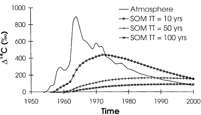
Figure 1. The time record of14C in the atmosphere (Northern Hemisphere) based on grapes grown in Russia (Burchuladze et al. 1989) for 1950–1977 and direct atmospheric measure-ments for 1977–1996 (Levin & Kromer 1997). We express radiocarbon data here as114C, the difference in parts per thousand (per mil or‰) between the14C/12C ratio in the sample compared to that of a universal standard (oxalic acid I, decay-corrected to 1950). All samples are corrected for mass-dependent isotopic fractionation to−25‰inδ13C. Expressed in this way,114C values greater than zero contain bomb-produced radiocarbon, and those with114C less than zero indicate that carbon in the reservoir has, on average, been isolated from exchange with atmospheric 14CO2for at least the past several hundred years. The14C content of a homogeneous, steady state C reservoir with turnover times of 10, 50 or 100 years is compared with that of the atmosphere through time.
tracer for C cycling on decadal time-scales. Carbon reservoirs such as SOM that exchange with the atmosphere reflect the rate of exchange through the amount of ‘bomb’ 14C incorporated (Figure 1).14C in atmospheric CO2 is
currently decreasing at a rate of about 8‰per year (Levin & Kromer 1997) because of uptake by the ocean and dilution by burning of 14C-free fossil fuels. The14C content of a homogeneous C reservoir in any given year since 1963 may be predicted from the turnover time and the known record of atmo-spheric 14CO2. Utilization of bomb-produced 14C as a continuous isotopic
label has advantages over other isotopic methods because it can be used in undisturbed ecosystems and can resolve dynamics that operate on annual to decadal time scales.
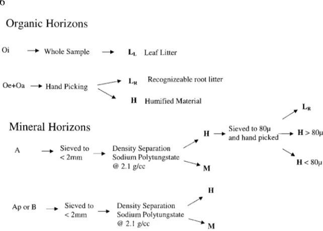
Figure 2. Schematic representation of soil sample processing into the homogeneous soil
organic matter pools as defined in this paper; LLor LR(recognizable leaf or root litter
respec-tively), H (undifferentiable SOM which is considered to be microbially altered or humified), and M (organic matter associated with mineral surfaces). All LL, LRand H components are
low density (i.e.<2.1 g/cc) while the M components are considered high density (i.e.>2.1 g/cc).
turnover times (see Figure 2): recognizable leaf (LL) and recognizable fine
(<2 mm) root litter (LR), organic matter that has been transformed by
micro-bial action or humified, but is not stabilized by interactions with mineral surfaces (H), and organic matter that is associated with soil minerals and thus is separable by density (M). These four pools collectively comprise Reservoir-C as defined for this paper and represent detrital C that remains in the soil for one year or more. Carbon pools in SOM that cycle on timescales of less than one year are included in our definition of Recent-C.
Carbon dynamics derived from measurements of 14C in SOM fractions
alone tend to underestimate the flux of CO2from soils. Heterotrophic
respira-tion is dominated by decomposirespira-tion of C with short turnover times and small reservoirs that are difficult to measure. The majority of easily measurable SOM stocks represent slowly cycling material with relatively long turnover times. Measurements of 14C in CO2 can be used to determine the relative
atmosphere profiles with a model of soil gas diffusion to determine the rate and14C signature of CO2production in soil by horizon. This, combined with
the predicted production of CO2and14CO2derived from the LL, LR, H and
M fractions of SOM, allowed us to partition soil respiration into Recent-C and Reservoir-C.
Site description
The Harvard Forest is a mixed deciduous forest located near the town of Petersham in central Massachusetts. The study area is located on the Prospect Hill Tract (42.54◦ N, 72.18◦ W). The terrain is moderately hilly (average elevation 340 m) and currently about 95% forested (Wofsy et al. 1993). The soils are developed on glacial till deposits which are predominantly granitic. Drainage varies from well-drained uplands, which make up most of the area in the flux tower footprint, to very poorly drained swamps. The data reported here are for well drained soils with very low clay content and mapped as Canton Series (coarse-loamy over sandy or sandy skeletal, mixed mesic Typic Dystrochrepts). We sampled soils, soil respiration and soil gas profiles within 100 meters of the eddy flux tower where a multi-year record of soil respiration measured by flux chambers is maintained (Davidson et al. 1998). The sites are within a mixed deciduous stand, dominated by red oak (Quercus rubra) and red maple (Acer rubrum) with some hemlock (Tsuga canadensis) and white pine (Pinus strobus). The area comprising our study site was cleared in the mid-1800’s, plowed and used primarily for pasture. The pasture was abandoned between 1860 and 1880 (Foster 1992). The regrowing forest was largely leveled by a hurricane in 1938 but has been growing undisturbed since that time.
Methods
Field
We sampled soils using the quantitative pit methodology as discussed by Huntington et al. (1989) and Hamburg (1984). This method involves sampling a large volume of soil to allow calculation of horizon-specific bulk densities. Two 0.5×0.5 m quantitative pits were dug in 1996 to a depth of about 80 cm. Pit locations were selected to be similar to those where Davidson et al. (1998) are monitoring soil respiration and soil CO2 concentrations and are within
by color and textural changes. In order to minimize sampling errors due to repeated grid placement and removal, the top of each pedogenic horizon was calculated by taking a weighted mean of 25 measurements from within the 0.5×0.5 m grid. This system weights the center nine measurements 4×, the sides of the grid (not including the corners) 2× and the corners 1×. Additional samples which integrated each soil horizon were collected for radiocarbon and total C and N analyses from one of the pit faces. Samples of the forest floor (0.15×0.15 m squares), core samples of A horizons and grab samples of Ap and B horizons were collected in order to analyze the abundance and14C of roots. During the summer of 1997, a third, shallower
(0.17 m×0.37 m) pit was dug to obtain more data for the O and A horizons. Samples were taken in approximately 2 cm vertical increments to the base of the Ap horizon.
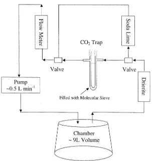
Collars sampled were the same as those used by Davidson et al. (1998) to monitor soil respiration fluxes. Closed dynamic chambers were used for sampling isotopes in soil respiration, as shown in Figure 3. First, atmospheric CO2initially inside the chamber cover was removed by circulating air at flow
rates of∼0.5 L min−1from the chamber headspace through a column filled
with soda lime. Scrubbing continued until the equivalent of two to three chamber volumes had been passed over the soda lime. Then the air flow was switched and flowed through a molecular sieve trap (mesh size 13×). Molecular sieve 13×traps CO2quantitatively at room temperatures and then
releases it when baked at 475◦C (Bauer et al. 1992). CO2was trapped from
circulating chamber air until the amount required for isotopic (13C and 14C)
measurements (∼2 mg of C) was collected. Trapping times varied from about 10 minutes to an hour, depending on the soil CO2emission rate. To achieve
100% yields of CO2 from the molecular sieve traps we have found that it is
important to put a desiccant in-line (Drierite) in order to minimize the amount of water getting to the molecular sieve
To measure CO2and its14C signature in the soil atmosphere we collected
soil gas samples from stainless steel tubes (3 mm OD) inserted horizontally into soil pit walls (the soils pits were subsequently backfilled). The air within the tubing was first purged by extracting a 15 ml syringe sample through a fitting with a septum. Two more 5 ml samples were then withdrawn from each tube, the syringes were closed with a stopcock, and the CO2
concen-trations of the syringe samples were analyzed the same day in a LiCor infrared gas analyzer as described by Davidson and Trumbore (1995). For the
14C analysis, we filled evacuated stainless steel cans (0.5–2.0 L volume) by
Figure 3. Sampling scheme for trapping CO2 on molecular sieve (mesh size 13×) using
a closed dynamic chamber system. Molecular sieve 13×traps CO2 quantitatively at room temperatures and then releases it when baked at 475◦C (Bauer et al. 1992). The evolved CO2
is purified cryogenically.
TDR and temperature probes in one pit in 1995 (not dug quantitatively for bulk density) and in a second pit dug in 1996 (dug quantitatively as discussed above). All pits were located within a few meters of each other. The concen-trations of CO2, water content, and temperature were measured weekly during
the summer, once every two weeks during the autumn and spring, and once per month during the winter.
Laboratory
Prior to C and14C analyses, soil samples were separated into different SOM fractions as defined for this paper (LL, LR, H and M) according to procedures
outlined in Figure 2. For mineral samples, material that was less than 2.1 g/cc was primarily humified material (H). Fine roots (LR) were a significant
component of low density organic matter only in the A horizon samples. To test for the importance of LR in determining bulk low density 14C values,
after density separation, one A horizon sample was sieved to 80µand then hand picked to separate H from LR components for 14C analysis. The Ap,
Bw1 and Bw2 horizons had such a small proportion of fine root material this additional processing was not performed. Once a soil C fraction was isolated, it was split and half the sample was archived while the other half was ground or finely chopped and analyzed for carbon and nitrogen content in a Fisons 5200 Elemental Analyzer. Grinding was done with an air cyclone sampler for the Oi horizon. Oe + Oa samples and root samples were chopped finely with scissors and mineral samples were ground by hand with a mortar and pestle.
In order to quantify fine root biomass, samples were taken by coring or from subsamples dug from our quantitative pits. Samples were frozen immediately after collection, then stored and processed at the Woods Hole Research Center. Oe + Oa horizons were thawed, a sub-sample removed (approximately 8 cm3) and quantitatively picked for fine roots (<2 mm in
diameter). Mineral soils were thawed, sieved through a 5.6 mm sieve and the fine roots that did not pass through the sieve were weighed. In order to pick live versus dead fine roots, a sub-sample of the sieved soil was used (approximately 8 cm3). Graphite targets of all SOM fractions and soil gas (CO2) were prepared at UCI using sealed tube zinc reduction methods
(Vogel et al. 1992). The14C analyses of these targets were made by acceler-ator mass spectrometry (AMS) at the Center for AMS, Lawrence Livermore Laboratory, Livermore, California (Southon et al. 1992). Radiocarbon data are expressed as114C, the per mil deviation from the14C/12C ratio of oxalic acid standard in 1950, with sample14C/12C ratio corrected to a δ13C value
of −25‰ to account for any mass dependent isotopic fractionation effects (Stuiver & Polach 1977). The precision for radiocarbon analyses prepared using the zinc reduction technique in our laboratory is±7‰for values close to modern (0‰).
We measured13C in a subset of our SOM samples to determine the proper
13C correction for calculating 114C values. Low density samples had δ13C
fractions, we used the same correction (−26‰) for all SOM. The maximum error introduced to our 14C determination by this assumption (5.1‰) is less than the analytical uncertainty of 7‰.
Measurements of13C for surface CO
2 flux samples were used to correct
for mass dependent fractionation as well as to correct for incomplete stripping of atmospheric CO2 in the chamber system during CO2 trapping. The δ13C
value for CO2 in air (δ13Catmosphere) is ∼ −8.5‰, whereas the δ13C of soil
respiration should be close to that of SOM (δ13C
soil = −26‰). The fraction
and we calculate the114C of the soil respiration:
114Csoil=
114C
measured−X×114Catmosphere
(1−X) . (2)
The value of δ13C
atmosphere at the level of the respiration collars (∼5–10
cm) can become as light as ∼ −11‰ due to atmospheric inversion which traps plant respired CO2 and any fossil fuel derived CO2 (particularly in
winter) near the surface. Therefore, during each sampling event we trap one air sample and analyze this for δ13C. The resulting δ13C is then used for
δ13Catmosphere in calculation of equations 1 and 2 for that suite of samples.
Values of X ranged between 0.09 and 0.61. The highest values of X are asso-ciated with the samples taken in May, 1996, when no attempt was made to strip the initial chamber of atmospheric CO2(values in May were 0.61, 0.49,
0.40 and 0.34). For the July, September and December sampling events when 2–3 chamber volumes were stripped prior to sampling, values of X were all below 0.31 with an average of 0.17.
Modeling
Our methods for data analysis involve four modeling components: 1) determi-nation of CO2production by horizon, 2) estimation of114C of CO2produced
within each horizon, 3) calculation of the amount of CO2 derived from
decomposition of Reservoir-C sources and 4) partitioning of soil respiration into Recent- versus Reservoir-C sources based on a C and14C mass balance
approach. Each modeling component is discussed in turn below.
(1) CO2production within each horizon
The production of CO2 within each horizon was calculated by combining
diffusivity was estimated for each soil horizon using the model of Millington and Quirk (1961), modified for the presence of rocks and for temperature:
Ds
where Ds is the diffusion coefficient in soil, Dois the diffusion coefficient of
CO2in air (0.139 cm2s−1at 273◦K at standard pressure),α is the total
air-filled porosity, ε is the total porosity, %RF is the percent rock fraction, and T is the soil temperature (◦K). As described by Collin and Rasmuson (1988)
and by Davidson and Trumbore (1995), the exponential term, 2x, is usually close to 4/3, and can be approximated by the polynomial
x=0.477α3−0.596α2+0.437α+0.564 (4)
The first term in the Millington and Quirk (1961) equation estimates diffusivity in the wet porous soil medium. The second term, which we have added here, adjusts for rock content of these glacial soils, assuming that diffu-sion of gases through rocks is negligible. The third term, adjusts for the effect of temperature on gaseous diffusion (Hendry et al. 1993). Total porosity is estimated as
where BD is bulk density of the<2 mm soil fraction measured in our quanti-tatively sampled soil pits, and PD is a weighted average of particle density, assuming that organic matter has a PD of 1.4 g cm−3and soil minerals have a PD of 2.65 g cm−3. Air filled porosity (α) was calculated as the differ-ence between total porosity and volumetric water content measured by time domain reflectometry (TDR) probes, as described by Davidson et al. (1998).
The soil CO2concentration profile was fitted to an exponential function
(Figure 4):
[CO2]z=CO2∞(1−e−βz)+0.04, (6)
where [CO2]z is the concentration of CO2 at depth z in percent, CO2∞ is
the fitted asymptotic CO2 concentration at infinite depth, z is soil depth in
cm, β is a fitted parameter, and 0.04 is an adjustment for the approximate concentration of CO2 at the soil surface (i.e., about 400 µL CO2 L−1 air).
The first derivative of this equation is used to estimate the diffusion gradient as a function of depth:
dCO2
dz =CO2∞×β×e
Figure 4. Calculation of CO2flux estimates by depth (Fz, where z indicates the profile depth)
and CO2production estimates by soil horizon (Ph, where h indicates the specific soil horizon) in gC m−2hr−1. The values shown here are from measurements made on 25 August 1997. Interpolations among similar measurements made throughout the year were summed to obtain annual estimates. These estimates are for well drained soils within the footprint of the eddy flux tower at Harvard Forest.
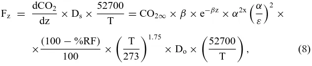
Applying Fick’s first law and combining equations, the flux of CO2at a given
depth (Fz) can be calculated from the product of the diffusion gradient and
the effective diffusivity:
Using this equation, the flux at the top of each mineral soil horizon (see Figure 4) was calculated for each sampling date in each of the two instru-mented soil pits. Our approach to calculating diffusivity differs from many others (e.g., de Jong and Schappert 1972; Johnson et al. 1994; Mattson 1995), in which the flux was calculated from an assumed linear diffusion gradient between two points where CO2 concentrations were measured. The
expo-nential fit used here for characterizing the CO2 profiles (Figure 4), while
Finally, estimation of the production of CO2within each genetic horizon
(Ph) was calculated from the difference between the flux at the top and bottom
of a given soil horizon such that
Ph=Fh−out−Fh−in, (9)
where Fh−outand Fh−incorrespond to the appropriate Fz (Figure 4).
Produc-tion within the O horizon was estimated by the difference between the mean of the six surface chamber flux measurements and the calculated flux at the top of the A horizon. This approach avoids the difficult problem of estimat-ing diffusivity in the O horizons, where small differences in measured bulk density and water content (both of which are difficult to measure well) would have a large effect on our estimate, and where diffusion may not always be the dominant mechanism of gas transport.
(2) 114C of CO
2produced within each horizon
The total CO2and 14CO2flux leaving a soil horizon results from a mixture
of the CO2that is diffusing through that horizon and that which is produced
within the horizon. Therefore, based on horizon specific estimates of CO2
production (Ph) and measurements of the14C in CO2 coming into (1Fh−in)
and going out (1Fh−out) of a subset of the soil horizons (in this notation, 1
refers to 14C of F in‰units, and not “change in F”), we can use a simple mixing equation to calculate the 14C of CO
2 produced within that horizon
(1Ph) from both Recent- and Reservoir-C sources. The equations used to
calculate1Ph(in‰units) from CO2production rates and fluxes (in gC m−2
yr−1) are Equation 9 and
(Fh−in+Ph)×1Fh−out=Fh−in×1Fh−in+Ph×1Ph (10)
In this approach chamber measurements of14C in CO2from the surface efflux
serve as1Fh−outfor the O horizon and are used to calculate1Phfor the entire
O horizon. We lumped O, A and Ap horizons (representing the top∼15 cm) because of the large variability in the14CO
2 data available for constraining
the O/A and A/Ap transitions.
(3) Decomposition of Reservoir-C
We calculate decomposition of Reservoir-C fluxes by first calculating turnover times for each SOM component using its 14C signature and then
calculating a decomposition flux based on that turnover time.
(3.1) SOM turnover times from14C
(Ap and B), we used a time-dependent, steady state model as presented in Trumbore et al. (1995):
C(t)×Rsom(t) = I×Ratm(t)+C(t−1)×Rsom(t−1)−k×C(t−1)×
×Rsom(t−1)−λ×C(t−1)×Rsom(t−1), (11)
collecting terms:
Rsom(t)=
I×Ratm(t)+(C(t−1)×Rsom(t−1)×(1−k−λ))
C(t)
, (12)
where:
C = Stock of carbon for the given C pool in gC m−2
I = Inputs of C above and below ground in gC m−2yr−1
k = Decomposition rate of SOM in yr−1
R = 1100014C−1
Ratm = The ratio of14C in the atmosphere normalized to a standard.
Rsom = The ratio of14C in the given SOM pool: L, H or M, normalized
to a standard.
λ = radioactive decay constant for14C = 1/8267 years.
t = time (year) for which calculation is being performed
I and k are adjusted to match both observed C inventory and14C content for the fraction in 1996. Note that the Rsomat any time t, depends not only on the
Ratm(t)but on both C inventory and Ratmof previous years.
For the Oe + Oa and A horizons that have accumulated above the plow layer since abandonment between 1860 and 1880, we used a nonsteady state model that matches both the total amount of C and14C in 1996. We assumed zero initial C in 1880. Assuming constant I and k, the amount of carbon initially added in each year j (since 1880) that remains and can be measured in 1996 (Cj) will be
Cj=I×e−k(1996−j), (13)
The 14C signature of C
j will be Ratm(j). Therefore the total amount of
carbon and radiocarbon measured in 1996 is shown by Equations 14 and 15, respectively:
C1996 = j=1996
X
j=1880
Rsom(1996) =
Again, I and k were adjusted until they matched observations of C and14C
for each fraction in Oe + Oa and A horizons. The rate of accumulation of carbon for a given fraction in 1996 is the difference in C inventory calculated for 1995 and 1996.
Both steady state and nonsteady state accumulation models assume (1) all carbon within a given SOM fraction (LL, LR, H, or M) is homogenous with
respect to decomposition; (2) the time lag between photosynthetic fixation and addition of fixed C to SOM is one year or less (i.e. the 114C of C
added to each SOM fraction each year is equal to Ratm(j)) and (3) radiocarbon
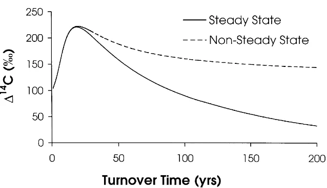
does not fractionate during respiration. We have already corrected for mass-dependent fractionation effects when calculating 114C values. Any time lag that does exist between photosynthetic fixation and addition of fixed C to SOM (contrary to Assumption 2) will cause an overestimation of turnover time (TT) equal to this lag (Thompson & Randerson 1999). Assumption 2 holds for the majority of aboveground litter inputs (deciduous leaves) which are fixed and fall to the ground within one year. Effects of this assumption with respect to other SOM inputs will be discussed later in the text. Figure 5 shows the114C of a SOM fraction as a function of turnover times in 1996 for both the steady-state and nonsteady state models. Significant differences between approaches appear only for fractions with turnover times greater than about 25 years. This is because the assumption of zero initial carbon in 1880 in the accumulation model limits the amount of pre-bomb 14C in the SOM
that is available to dilute the post-bomb carbon that has accumulated since 1963.
(3.2) Calculating SOM decomposition fluxes
Decomposition fluxes for the LL, H and M components of SOM are
deter-mined as the inventory in each fraction divided by the turnover time derived from14C. Since the turnover times for fine roots are too uncertain (as will be discussed in the results section), we treat the flux from LRas an unknown and
solve for it in the C and14C mass balance section.
The turnover times derived from 14C data may represent the time scales for C loss via several mechanisms, including (1) decomposition loss of CO2
Figure 5. The predicted 114C value in 1996 for homogeneous C reservoirs as a function of turnover times. The curves represent results for our steady state and nonsteady state (accumulation) models.
for dissolved organic carbon (DOC) transport from similar stands in Harvard Forest are available from Currie et al. (1996), and show leaching losses to be minor compared to the other fluxes, except in the O horizon where DOC loss is approximately 20 gC m−2yr−1. This loss is only a few percent of the total annual CO2 flux, hence we have excluded it from consideration here.
Consequently, we assume all loss to be from decomposition or transfer from one C fraction to another.
We model the litter components LL and LR as having two fates:
decom-position to CO2or transfer to the H or M fractions. For the H and M fractions
we assume that their source of C is transfer from LL and LR fractions and
that their most important loss process is decomposition to CO2. The flux of
CO2derived from decomposition of leaf litter (FLL) is the inventory of leaf C
divided by its turnover time, corrected for the fraction of LLthat is transferred
to the H + M pools. Since we cannot independently partition the flux of LL
into either CO2or a transfer flux, we bracket our estimates by assuming two
extreme cases in which all of the H + M inputs come from either (1) LLor (2)
LR.
(4) Partitioning of soil respiration sources
The total amount of radiocarbon in soil respiration equals the amount of CO2
one year). If the 114C signatures of these components differ significantly,
we may use a mass balance approach to determine the relative contribution of each to total soil respiration. We use an isotopic mass balance based on estimates of CO2 production, the 114C in CO2 and 14C-derived estimates
of decomposition fluxes from the SOM fractions. For the whole soil profile, equations of mass balance for C and14C are
P=FR+FLL+FLR+FH+FM (16)
and
P×1P = FR×1Ratm(1996)+FLL×1LL+FLR×1LR+
+FH×1H+FM×1M. (17)
In Equations 16 and 17, P is the total annual soil respiration flux and FRis the
flux of CO2derived from Recent-C. FLL, FLR, FH and FM are fluxes of CO2
derived from their respective Reservoir-C sources. The 1 values required for the 14C mass balance are either measured (for 1LL, LR, 1H and1M),
assumed to equal 1Ratm(1996) (for Recent-C), or calculated from CO2 and 14CO
2fluxes (1P). For the soil profile as a whole, P and1P are the measured
surface flux and its114CO
2signature respectively.
We then solved Equations 16 and 17 for the remaining unknowns, FRand
FLR. Since C stocks and rates of C turnover vary vertically within the soil
profile, the relative proportions of CO2from FRversus the SOM fractions will
vary with soil depth and horizon. Equations 16 and 17 may also be written and solved for each individual soil horizon. However, because of difficulties in characterization of the O/A horizon transition, and uncertainties in the production of roots as a function of depth, we have combined the O + A + Ap horizons and performed the14C mass balance on only three layers: the O + A + Ap (uppermost 15 cm of soil), B and C horizons.
Results
Carbon inventory
49
Low density SOM High density SOM Bulk Soil Bottom Total Leaf litter Fine root Humified Mineral associated density1,2 carbon3 depth4 C stock5,6 LL7,8 detritus LR7,8 H8,9 M8
Horizon (g cm−3) (gC Kg−1soil) (cm) (gC m−2) (gC m−2) (gC m−2) (gC m−2) (gC m−2)
Oi 0.06 (0.01) 450 (20) 2 (1) 380 (110) 380 (110) 0 – NA Oea 0.1 (0.02) 470 (10) 6 (1) 1640 (750) – 230 (40) 1410 (750) NA A 0.35 (0.03) 270 (30) 10 (2) 2400 (820) – 60 (25) 1780 (630) 560 (200) Ap 0.54 (0.13) 60 (1) 16 (2) 2620 (660) – 70 790 (200) 1760 (450) Bw1 0.85 (0.07) 20 (1) 32 (4) 1245 (190) – 4 40 (10) 1200 (180) Bw2 0.93 (0.04) 6 (1) 59 (3) 510 (110) – 1 (1) 5 (1) 500 (110)
Total 8800 (1310) 380 (110) 360 (70) 4030 (1000) 4020 (540)
1 Gravel free bulk density (i.e. less than 2 mm).
2 For Oi, Oe + Oa and A horizons n = 3, standard error in parenthesis; n = 2 for all other horizons; range in parenthesis. 3 For all horizons n = 2; range in parenthesis.
4 For Oi, Oe + Oa and A and Ap horizons n = 3, standard error in parenthesis; n = 2 for all other horizons; range in parenthesis. 5 Includes live root mass below the Oi horizon; total error in parenthesis.
6 C stock calculated using a z value (not shown) that accounts for waviness of horizon boundary and rocks.
7 On a dry weight basis; error term includes extrapolation from subsample to whole soil where subsample n = 3 to 5, otherwise n = 1 and no
error is shown.
(80%) in the upper 15 cm, which make up the organic and A + Ap horizons. Measured litterfall inputs to the O horizon were 150 gC m−2yr−1in 1996.
The fraction of soil volume taken up by rocks is spatially variable. In two of the three pits the O and A horizons were much less rocky (0–2% rocks) than the B horizons (10–35% rocks). However, one of our three pits had no less than 15% rocks in all horizons down to 60 cm. Spatial heterogeneity in soil C stocks has been studied in rocky forest soils similar to those found at Harvard Forest. Fernandez et al. (1993) show that between 73 and 455 samples are required to quantify C stocks to within 10% depending on soil depth. Huntington et al. (1988) were able to quantify C stocks to within 20% only after digging 60 0.74×0.74 m pits. Therefore in this study instead of quantifying variability within a site we focus on the C dynamics for specific profiles and assume C dynamics will be the same even if the inventory of a given SOM fraction varies spatially for sites with similar drainage.
The four rightmost columns of Table 1 show the inventory of the isolated soil C fractions LLor LR, H and M. Carbon in low density fractions decreases
rapidly with soil depth, from 100% in O horizons to<1% in B horizons. Low density carbon (LL + LR+ H) makes up 54% of the total soil carbon stock,
but is 87% of the carbon in O + A horizons.
Quantitative picking of roots showed they make up 7–19% (n = 5) and 1–4% (n = 5) of the dry mass in the Oe + Oa and A horizons, respectively. Assuming roots are 50% C by weight, the fraction of carbon in live and dead roots make up∼14% of the total C stocks in the Oe + Oa horizon, decreasing to∼0.2% in the Bw2 horizon. Our estimate of total fine root mass of 360 gC m−2(live + dead) is lower than that of McClaugherty et al. (1982), who found 525 gC m−2(live + dead) in well-drained mixed hardwood soils at a neighboring study area within the Harvard Forest. Fahey and Hughes (1994), found∼320 and 350 gC m−2(live + dead) in June and October respectively in a mature northern hardwood forest. Our values also decrease more rapidly with depth than those of McClaugherty et al. (1982) who found 70, 55, and 15 gC m−2for 15–30, 30–45 and>45 cm respectively for live + dead fine roots. In addition, our ratio of live:dead fine roots (data not shown) at all depths are significantly greater than those reported by McClaugherty et al. (1982), suggesting either differences in procedures for distinguishing live from dead roots or that we sampled during a seasonal maximum in live root abundance. Technically, it is the dead roots, not the live roots, that are decomposing and contributing to CO2fluxes. Therefore, live roots should not be considered part
CO2production estimates
Total soil respiration as determined from chamber measurements in 1996 was 840 gC m−2yr−1 (Davidson & Savage, unpublished data). Production rates for CO2(Figure 4) by soil horizon were 190, 340, 235 and 75 gC m−2yr−1
for the O, A + Ap, B and C horizons respectively. The estimates of CO2
production within each soil horizon include uncertainties associated with the diffusion model, the exponential fit of the CO2concentration profiles, and, in
particular, measures of rock content. We used the average rock content of two quantitatively sampled soil pits dug in 1996. One had almost no rocks in the O and A horizons while the other had 20–30% coarse fragments. Repeating the calculations assuming either no rocks or the higher estimate of rock content, changed CO2production rates for the A horizons by roughly 50 gC m−2yr−1.
Radiocarbon in SOM fractions
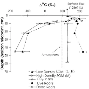
The average radiocarbon content and the range of values measured in the isolated SOM fractions are plotted by horizon in Figure 6.114C values for the low density SOM (LLor H) fractions increase from the Oi horizon (LL) where
values are 132±8‰to a maximum in the Oe + Oa horizon (H) of 200±19‰. Humified material in the A horizon is 121‰, and its14C signature decreases
rapidly in the Ap and B horizons. Within all mineral horizons, the low density carbon, which is primarily humus (H), has consistently higher 114C values
than mineral-associated (M) carbon, with the largest difference (55‰) in the Ap horizon. Large negative 114C values in both H and M fractions in the
Bw1 and Bw2 horizons indicate the majority of soil carbon at these depths has not exchanged with the atmosphere since 1950 and has, in fact, remained in the soil long enough for significant radioactive decay to occur (half life = 5730 years).
The 114C content of live and dead fine roots by horizon are also shown
in Figure 6. All roots have114C values between 134 and 238‰, significantly higher than the atmosphere or live deciduous leaves sampled during 1996 (97±7‰). Live roots on average have lower114C values than dead roots, and
Figure 6. 114C of below ground soil organic matter fractions and CO2by depth. All values
except the114C of CO2are plotted at the midpoint of the soil horizon. For the soil organic
matter fractions LL, H and M, the error bars represent the range (n = 2) or the standard error of
the mean (n = 3). For live and dead roots, the error bars where present, represent the error of the mean (n = 3) otherwise n = 1. For the soil CO2profiles values are an annual concentration
weighted mean (n = 3 or 4) with error bars showing the entire range of values measured. The surface flux represents a flux weighted annual average from four sampling events. The114C for the atmosphere for 1996 (97±1‰) is also shown.
still significantly higher than the atmosphere in 1997 (92±7‰), confirming that at least this one live root contained relatively “old” carbon. This one root may not be representative of all species and growth forms, which were averaged during the 1996 quantitative root picking.
The 1997 root data show that different parts of the same root have C that differs in age by 2 years. Thus, if longer turnover is the explanation for elevated14C, fine roots even 1 mm in diameter and less may not be acting as a single pool with one TT. The data would then imply that the tips (a small part of the mass) may turn over significantly faster than the rest of the root (the bulk of the mass). In a manner analogous to SOM stocks, the most recalcitrant root biomass pool is the largest fraction of the total root biomass pool and is the portion most easily separated from a soil sample for analyses.
Presently, we do not know which of the three above hypotheses for explaining high 114C values in root biomass is correct, and additional research is being conducted to address this important issue. We can however, proceed with our mass balance approach without calculating any turnover times for fine roots based on their 114C values. We instead solve for FLR
as one of the unknowns. However, even without an understanding of the mechanism, our 114C data show that live fine roots, upon their death, are adding carbon to SOM that averaged roughly 165‰ in 1996 and that must have been fixed on average 7±1 years previously.
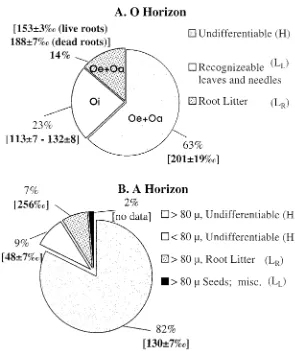
Figure 7 shows the distribution of C and 14C among the different low
density components in O and A horizons. In the O horizon (Figure 7(A)), deciduous leaf parts had114C values that increased with depth, from 113‰
in the Oi to 132‰in the Oe + Oa, where leaves became difficult to recog-nize. Radiocarbon in fine roots, which represent 14% of O horizon C (Table 1), ranged from 153‰ (live roots) to 188‰ (dead roots). The remaining, undifferentiable, material (H) had a114C value of 201±19‰(n = 2). Visual inspection shows H, which contained 63% of C in this O horizon sample, consisted of extremely fine root fragments (<0.5 mm), and dark, humified material that could not be identified.
Figure 7(B) shows the distribution of C and114C for the A horizon low
density fraction, which was sieved to 80µand hand picked to remove roots. The measured components range in value from 48‰to 266‰. The>80 µ
material makes up 82% of this low density sample and has a114C of 130‰. Roots (live + dead) are 7% of the carbon with a weighted average114C of
256‰(n = 2). The<80µfraction had the lowest measured14C value (48‰). The inventory-weighted average 114C for all four components was 132‰.
Figure 7. Heterogeneity of the O (top, Figure 7(A)) and A (bottom, Figure 7(B)) horizons. An
error of 7‰indicates analytical error, as n = 1. Errors other than 7‰indicate either a range (n = 2) or standard error of the mean (n = 3). Values for the O horizon (Figure 7(A)) represent a composite of several samples and are representative of an average O horizon. Values for the A horizon in Figure 7(B) represent the results of quantitative sieving and picking one sample as outlined in Figure 2. The roots in the A horizon represent a stock weighted mean of two samples representing roots of two morphological types with values of 231±7‰and 266±7‰.
Radiocarbon in the 1996 atmosphere at Harvard Forest
Partitioning of soil respiration using isotopic mass balance requires that we know the 114C of CO
2 for the atmosphere in 1996 (variable1Ratm(1996) in
a live deciduous leaf collected on the same date. The three values are 98±7, 96±6 and 97±7‰, averaging 97±1‰. We assume the C lost within a year of being fixed by photosynthesis, including root respiration and decomposition of labile SOM, will have this value in 1996. We support this asssumption with two lines of evidence. First, Horwath et al. (1994) performed a whole tree labeling study on two year old, three meter tall tulip poplar trees. They found that respiration of labeled C from the roots occurred within 12 hours of labeling, the peak activity in respiration was measured after two days and within two weeks the activity of root respiration was less than 5% of the maximum value. Second, three fruiting bodies of the genus Boletus, a mycorrhizal fungal symbiont, collected in 1996 at Harvard Forest had114C of 97, 99 and 98‰. The fact that their114C signature is the same as the 1996 atmosphere, indicates they are living off of Recent-C substrates, namely root exudates, and not the relatively 14C enriched Reservoir-C of the O horizon in which they are rooted. Since root exudates are Recent-C it follows that maintenance metabolism by trees in this ecosystem must also be respiring Recent-C.
Radiocarbon in soil CO2
Figure 8(A) and (B) shows CO2 fluxes and measured 114C in CO2 of the
surface flux for four sampling periods in 1996. The CO2 fluxes shown in
Figure 8(A) range between 40 and 200 mgC m−2 hr−1. The largest values
measured were in the early summer and the lowest in the winter (see Davidson et al. (1998) for more complete seasonal CO2 flux data). All flux
measurements were made within 1–2 days of 14C sampling, except for the
late September sampling event when fluxes were measured 8 days previously. Measured114C in CO
2values for 1996 in Figure 8(B) range from 103–176‰
and are all higher than the atmospheric 114CO2for 1996 (97±1‰). Hence,
decomposition of organic matter in the LL, LRand H fractions, primarily in
the O and A horizons, and which have114C values greater than 100‰, must contribute significantly to the total soil CO2flux. In 1996, the highest114C
values in soil respiration were observed in the spring and summer with values of 138 and 149‰ respectively. The lowest values were in fall and winter where114C drops to 111 to 121‰respectively. The data from Figure 8(A)
and (B) were used to calculate an annual flux weighted mean 114C in soil respiration for 1996 of 128±9‰(n = 11).
The concentration-weighted annual average114C in CO2for soil air (by
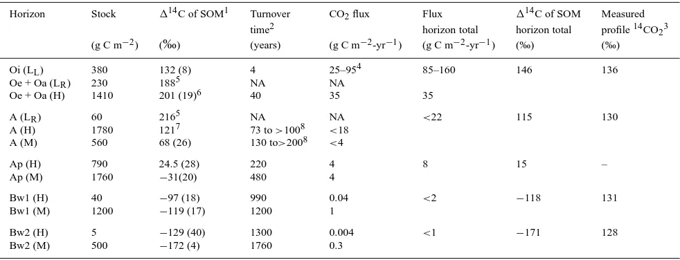
Table 2. Calculation of high and low density decomposition fluxes with associated114CO2and measured profile114CO2. Horizon Stock 114C of SOM1 Turnover CO2flux Flux 114C of SOM Measured
time2 horizon total horizon total profile14CO23
(g C m−2) (‰) (years) (g C m−2-yr−1) (g C m−2-yr−1) (‰) (‰)
Oi (LL) 380 132 (8) 4 25–954 85–160 146 136
Oe + Oa (LR) 230 1885 NA NA
Oe + Oa (H) 1410 201 (19)6 40 35 35
A (LR) 60 2165 NA NA <22 115 130
A (H) 1780 1217 73 to>1008 <18 A (M) 560 68 (26) 130 to>2008 <4
Ap (H) 790 24.5 (28) 220 4 8 15 –
Ap (M) 1760 −31(20) 480 4
Bw1 (H) 40 −97 (18) 990 0.04 <2 −118 131
Bw1 (M) 1200 −119 (17) 1200 1
Bw2 (H) 5 −129 (40) 1300 0.004 <1 −171 128
Bw2 (M) 500 −172 (4) 1760 0.3
NA = Not applicable, see text for details. – = no data.
1 Values are the average for two pits with range in parenthesis.
2 A nonsteady state model is used for the Oe + Oa and A horizons and a steady state model used for Oi, Ap and deeper horizons. 3 Represents an annual concentration weighted average of the measured114C in CO
2at the boundary with the horizon below. 4 Represents a range based on assuming all loss is as CO
2or that 100% of inputs to the H + M fractions are from leaf litter. 5 Represents the114C samples picked for dead roots (n = 1).
6 Represents the humified organic material after quantitative root picking for the Oe + Oa (n = 2).
Figure 8. CO2fluxes for 1996 (top, Figure 8(A)). Error bars represent standard error (n = 6). 114CO2of soil CO2efflux (bottom, Figure 8(B)) Error bars where present represent standard
error (n = 3) except in December 1996 where n = 1.
depths the annual variation was 20‰or less. The fact that the 114C in CO 2
is greater than either atmospheric CO2or H and M carbon in the mineral Ap
and B horizons shows decomposition fluxes must be dominated by root litter (FLR) which has much higher114C values.
Fluxes and turnover time of C in SOM fractions
values (>100‰) have two possible turnover times for each114C value. For
example, the114C of H in the Oe + Oa horizon is 201‰which corresponds to turnover times of either 9 or 40 years (Figure 5, nonsteady state model). Based on the requirements for total CO2and14CO2production in each horizon, we
chose the longer turnover time for the H fraction in this and other horizons. We did not calculate turnover times for root litter (LR) because of the potential
for a significant lag time to affect the114C values measured in 1996. The time lag would also affect the TT for undifferentiable (H) material that is derived from both leaf litter and fine roots. In each case, failure to correct for any lag will cause overestimation of turnover times by as much as the inferred 14
C-derived lifetime of live roots (7±1 years). Failure to account for time lags if roots are the principal source for more recalcitrant organic matter would result in turnover times for H and M fractions that are∼7 years too long.
The flux of CO2derived from decomposition of LL, H and M fractions is
calculated in Table 2 from the C inventory and turnover time. Again, no flux is calculated for fine root decomposition (FLR); instead we use the CO2 and 14CO
2mass balance to calculate this below.
Partitioning of soil respiration
Equations 16 and 17 contain three unknowns: FLL, FLRand FR. We therefore
introduce an additional constraint so that we may solve for all three fluxes. As we have defined them, LLand LRpools represent the detrital root and leaf
material that take longer than one year to decompose and are identifiable in SOM. From the inventory of detrital leaf litter (LL; 380 gC m−2) measured in
the soil, and its turnover time (4 years; Table 2), we calculate the annual flux of C into the LLpool as 95 gC m−2yr−1. The fate of leaf detritus is either to
decompose directly to CO2(this is the flux FLL) or to be incorporated into soil
humus and mineral pools (H + M). We do not know this partitioning; however, based on C and14C inventory and our nonsteady state model, we assume the
the annual rate of input to the H + M pools equals the decomposition flux from these pools (∼70 gC m−2yr−1, see Table 2). We then consider the two extreme cases, where all humus and mineral C is derived from leaf detritus, or all of it is derived from root detritus. FLLis thus constrained to be between
25 and 95 gC m−2 yr−1. In Table 3, we use these minimum and maximum
values for FLL and solve for the two remaining fluxes, FLRand FR. Table 3
also shows cases for using the minimum and maximum values for observed
114C of detrital leaf (113 and 132‰) and root (180 and 214‰) pools. The ranges and means of this approach are shown in Figure 9.
Our results from partitioning soil respiration for the entire soil profile using CO2and14CO2mass balance are summarized in Table 3 and Figure 9.
59 Case Parameters Leaf litter Leaf litter Fine root Fine root Recent-C Reservoir-C Recent-C Reservoir-C
F1
LL 1L2L litter FLR litter1LR3 FR FLL+ FLR+ FH+M fraction fraction
(gC m−2yr−1) (‰) (gC m−2yr−1) (‰) (gC m−2yr−1) (gC m−2yr−1)
Case 1 Min LL, min1LL, min1LR 25 113 277 180 470 370 0.56 0.44 Case 2 Min LL, min1LL, max1LR 25 113 197 214 550 290 0.66 0.34
Case 3 Min LL, max1LL, min1LR 25 132 272 180 475 365 0.57 0.43
Case 4 Min LL, max1LL, max1LR 25 132 193 214 554 286 0.66 0.34 Case 5 Max LL, min1LL, min1LR 95 113 264 180 413 427 0.49 0.51
Case 6 Max LL, min1LL, max1LR 95 113 187 214 490 350 0.58 0.42
Case 7 Max LL, max1LL, min1LR 95 132 242 180 435 405 0.52 0.48
Case 8 Max LL, max1LL, max1LR 95 132 172 214 505 335 0.60 0.40
Average 60 219 493 347 0.59 0.41
Minimum 172 413 286 0.49 0.34
Maximum 277 554 427 0.66 0.51
For all scenarios,114C of the atmosphere (1R) = 97‰, the114C of total soil respiration (1P) = 128‰, the flux of H + M is 70 gC m−2yr−1with a 114C of 135‰. We combine the fluxes and their associated14C values of the H and M pools because their combined fluxes are relatively low (less than 10% of the annual total). Nonbold face values are parameters used in Equations 16 and 17, while bold faced values are the resulting calculations.
1 Range reflects the two cases where either none or all of the inputs to H + M fractions are derived from leaf litter. 2 Range is for the lowest and highest measured values of recognizeable leaf parts.
Figure 9. Results of isotopic mass balance approach to partitioning soil respiration into
Recent- versus Reservoir-C sources. Solid arrows represent fluxes of organic C, while dashed arrows represent fluxes of CO2. All units are in gC m−2yr−1with the average (and range).
Production of litter (leaf and root) is assumed to have the isotopic composition of the atmo-sphere (97‰) in 1996. Bold numbers represent direct results from isotope mass balance model. Italicized numbers are independent measurements or calculated values used to constrain the model (see text for details) and underlined numbers are the resultant fluxes and transfers due to the model results and its constraints.
decomposition of low density SOM with TT greater than one year (LL, LR,
H and M, i.e., Reservoir-C). The decomposition of H and M fractions with turnover times>40 years contributes only 8% of the total annual respiration flux, with the remaining 33% (26%–43%) from root and leaf litter decompos-ition (with plant + soil residence times of 2 to 10 years). The fluxes into and out of the H + M pools are constrained by their14C-derived TT and reservoir size (Table 2) and represents an average over decadal time scales. The average flux of 70 gC m−2 yr−1 shown in Figure 9 implies the H + M pool to be in
steady state. The uncertainty of 40–70 gC m−2yr−1 is an estimate based on accumulation rates discussed in the following section.
Note that the flux of C into and out of the LL pool is less than the total
annual measured leaf litterfall (150 gC m−2yr−1; Figure 9). We infer that 55
gC m−2yr−1(1/3rd) of the freshly deposited litter is decomposed in<1 year (and hence is not detected from leaf detritus collected the following summer). Similarly, comparing the range of fluxes of C out of the LRpool (170–270 gC
m−2yr−1, which is equal to FLR+ the flux of root C transformed to humus)
Table 4. Summary of respiration partitioning results.
Horizon Total respiration Fraction total Fraction produced Min Max (gC m−2) respiration that is Reservoir-C
Whole Soil 840 1.00 0.41 0.34 0.51
O + A + Ap 530 0.63 0.44 0.35 0.54
B 235 0.28 0.39 0.32 0.45
C 75 0.09 0.37 0.31 0.43
gC m−2yr−1 indicates that 0–100 gC m−2yr−1of root litter is decomposed in less than one year.
Depth-dependence
Figure 4 and Table 4 show that 310 gC m−2yr−1or 37% of the total annual soil respiration is produced below 15 cm within the B and C horizons. Comparison of isotopic data for the SOM fractions in these horizons in Figure 6 and Table 2 clearly demonstrates that the two main sources must be root decomposition and Recent-C, because the decomposition of H + M reser-voirs accounts for<2 gC m−2yr−1(with FLL= 0). Application of C and14C
mass balance to the B and C horizons shows that 39% and 37% respectively, of the respiration comes from Reservoir-C (Table 4) and that essentially all of this flux is decomposition of roots with high114C values relative to the atmosphere. In the upper 15 cm of the soil profile (O + A + Ap) we estimate that 44% is Reservoir-C, with 32% from the decay of leaves and roots with TT of 2–10 years, and 12% from H and M fractions with TT >40 years. More frequent measurements of 14C in total soil respiration and within the vertical profile will allow for more detailed calculation of depth dependence of the make-up of soil respiration. Our measurement of root biomass in the B horizon (Table 1) is insufficient to support the approximately 90 gC m−2yr−1 of decomposition required by the mass balance approach, if fine root mass is homogenous with respect to turnover.
Discussion
Rate of carbon accumulation in SOM
The O and A horizons have accumulated 4.4 kgC m−2 above the plow layer
(leaf and root litter), which make up 15% of the soil carbon in these horizons, must have achieved steady state with vegetation inputs by 1996. Most of the C in the O and A horizons, however, is in the form of altered, humified (H) material not associated with minerals. The rate of turnover of these fractions is slow enough (40 to 100+ years) that the annual C inputs (I in Equations 11–13) required to support the inventory and14C observed in 1996 are small
(20–50 gC m−2yr−1in the Oe + Oa and 10–30 gC m−2yr−1in the A horizon. The rate of C accumulation in 1996 estimated using our accumulation model is 2–7 gC m−2yr1for the Oe + Oa and 8–23 gC m−2yr−1for the A horizon. The ranges reported bracket the values obtained for different model runs representing mean, low and high values (i.e.±1 standard deviation) of both C stocks (Table 1) and their14C values (Table 2). Also included in the range are runs done using the specific C inventories and114C values for each of
the two pits (data not shown). Variability in rock content between the two pits affected the overall C stock calculated for each pit and thus the pit with the most rocks had the smallest rates of C accumulation.
While these rates are large compared to storage rates in soils over longer timescales (e.g. Schlesinger 1990; Harden et al. 1992), they are less than the annual net C uptake measured for this ecosystem of∼200 gC m−2yr−1 (Goulden et al. 1996). Overall C accumulation rates by the well drained soils which dominate the area within the tower footprint account for 5–15% of this net ecosystem uptake. The predominant wind directions at the tower site are southwesterly and northwesterly. A small area of poorly drained soils close to the tower to the southwest and a swamp 500 m from the tower to the northwest could be larger sinks per unit area than are the well drained soils.
We have assumed the leaf and root litter pools, which have TTs<10 years, are at steady state. However, if net primary productivity has been increasing as a result of CO2 or N fertilization, then leaf and root litter pools may be
sequestering C. As discussed earlier, annual inputs to LL and LR pools are
150 and 270 gC m−2yr−1(see Figure 9). Assuming a 1% per year increase in NPP between 1991 and 1996 and correcting for the inputs respired during the same year then the LLand LRpools could also be storing a combined∼20 gC
m−2yr−1 ((270−15) + (150 −55)) gC m−2yr−1∗0.01 yr−1∗5 yr) through this period. Combined with the accumulation in the humic fractions of the O and A horizons this could account for as much as 25% of the net ecosystem uptake.
Partitioning of soil respiration
root respiration (plus decomposition of roots killed during trenching) was 33% of the total soil respiration at a nearby study site at the Harvard Forest. Using litterfall exclusion and addition manipulations, these authors estimate that 11% of the total soil respiration was from above-ground litterfall less than one year old. Hence, Bowden et al. (1993) estimated a total of 44% of the respiration was derived from C with a residence time in the soil system of less than one year. Both radiocarbon measurements and root and litter manipulations have uncertainties, and the best interpretation is probably that these two very different approaches yield estimates that about 50%±10% of the soil respiration is derived from C that is less than one year old. Bowden et al. (1993) also estimate that 30% of soil respiration was from root litter that had resided in the soil more than one year, which is consistent with our radiocarbon data that show somewhat surprisingly long mean residence times for live and dead roots.
Time lags in the soil C reservoir – potential for interannual variability
The measured114C of total soil respiration is 128±9‰for 1996 which corre-sponds to a mean residence time for C in the plant + soil system of 4±1 years. This represents the time an average C atom spends in the plant + soil system since original photosynthetic fixation and includes both root respiration and all decomposition sources. We also calculate the average value for114C of heterotrophic respiration is 167‰ which corresponds to an average age of 8±1 years. Thus a significant time lag exists between initial C fixation and ultimate respiration by heterotrophs. Therefore, variations in C storage or loss in any one year must partially reflect the net ecosystem uptake of previous years. (Schimel et al. 1997; Fung et al. 1997).
The age of C respired from soil can be used to predict the 13C isotope
disequilibrium for Harvard Forest. The 13C isotope disequilibrium is the difference between the 13C signature of atmospheric CO
2 being fixed by
plants and the 13C respired from soils. A difference is expected because the
13C in the atmosphere has been decreasing with time due to the addition of 13C-depleted fossil fuels to the atmosphere (e.g. Ciais et al. 1995; Fung et al.
1997). Using theδ13C trend of−0.02‰per year (Fung et al. 1997), and an average age of 8±1 years for heterotrophic respiration, we estimate the13C
at Oak Ridge, TN. Further work should place more emphasis on measuring radiocarbon in CO2respired from decomposing logs to asses the importance
of this component to total soil respiration.
Heterogeneity issues
Comparison of the bulk SOM114C with the114C in CO
2at depth (Figure
6) clearly demonstrates that the 114C signature of the SOM alone is not enough to estimate C dynamics. Even with density separations into low and high density pools, 114C of SOM is usually biased toward recalcitrant C stocks. This is particularly true in the mineral horizons where the vast majority of C stocks are hundreds of years old and have large negative114C
values. The small pools of fast cycling SOM (fine roots) with significant amounts of ‘bomb C’ are effectively diluted beyond isotopic recognition. Our technique of respiration partitioning, which accounts for decomposition via
14CO
2 measurements, is particularly robust in the mineral horizons where
the respiration sources are so isotopically different and have less spatial and temporal heterogeneity.
Methods of estimating bulk soil turnover rates by taking soil C stock divided by CO2flux also do not account for soil profile heterogeneity.
Particu-larly in temperate forest soils with significant O and A horizon carbon stocks, this approach will yield poor estimates of the response time of soils to climate change scenarios. Figure 10 shows differences in soil C increase in response to a 10% increase in C inputs for a one-pool model with a turnover time of 25 years versus a multi-pool model representing the well drained soil at Harvard Forest. The one pool model overestimates the amount of C sequestered both in the short and long term. After 100 years, the one-pool model over predicts C storage by almost 600 gC m−2.
Similarly, bulk SOM radiocarbon measurements may also cause an over-estimation of decadal scale SOM response. For example, had we not parti-tioned the low-density carbon in the A horizon into different components (fine roots, undifferentiable material >80 µand <80µ), the bulk14C value would have been 132‰with a TT of 66 years. Instead, Figure 7B shows the sample to be composed of components with 14C-derived TTs ranging from
∼8 to>100 years. Analogous to taking an average TT for the whole soil, the response of SOM would be overestimated if the114C signatures of the low-density C sample components were represented using the bulk radiocarbon value (see Figure 10).
Figure 10. Increase in C storage associated with a 10% increase in NPP for two non-steady
state models based on a one pool or four pool representation of soil organic matter stocks. In the one pool case the TT is 25 years and is equivalent to the total soil carbon stocks (8800 gC m−2) divided by the total soil respiration (840 gC m−2yr−1) multiplied by the amount of decomposition from Reservoir-C (41%). In the four pool case stocks and TTs are modeled after those for the Harvard Forest well drained soils with TTs of 1, 4, 80 and 500 years. Both systems are not at steady state; the increases are relative to a nonsteady state run for each case.
relative to 1996) was 660 gC m−2 yr−1 (Davidson & Savage, unpublished
data), compared to 840 gC m−2 yr−1 for 1996. Monitoring of soil respira-tion isotopic composirespira-tion should shed light on whether the reducrespira-tion in soil respiration in future years is caused by changes in decomposition, changes in root respiration, or both. The power of coupling this approach to measuring soil profiles of CO2and14CO2will allow determination of where in the soil
profile changes occur in response to climate.
Conclusions
• SOM pools are accumulating C in well-drained Harvard Forest soils as they recover from historic disturbance. However, the rates of accumula-tion we infer, 10–30 gC m−2yr−1, are only 5–15% of the 200 gC m−2 yr−1observed by the eddy flux tower. More poorly drained soils also in
the tower footprint may be accumulating larger amounts of C per square meter area, although they are far more limited in areal extent.
• Measurements of14C in soil organic matter emphasize organic matter
by estimated heterotrophic respiration are not good predictors of the response time of soils because soil organic matter (SOM) is not homo-geneous.
• Measurements of114C in CO
2are required to correctly model the C that
is actually respiring and to fully understand below ground C dynamics.
• Interpretation of14C data in SOM at Harvard Forest are complicated by
fine root inputs with14C elevated by∼65‰relative to the atmosphere, implying that the fine root C was fixed on average 7±1 years ago. We do not currently understand the mechanism behind this lag in radiocarbon input.
• We estimate 41% of total soil respiration comes from decomposition of SOM that decomposes on timescales of 1–100+ years. Of this, 80% involves direct decomposition of leaf and root litter with TT of 2–10 years and 20% represents low density humified C pools and C associated with minerals (H and M respectively) which have TTs on the order of several decades or greater.
• About two-thirds of total soil respiration is produced within the O and A horizons. These organic rich horizons are comprised of (1) small pools of live roots and recent leaf and root litter that have residence times in the plant + soil system of∼1–10 years and (2) relatively large pools of humified root and leaf litter which reside in the plant + soil system for 40–100+ years.
• Radiocarbon measurements of total below ground respiration measure the average time C spends in the plant + soil system from original photosynthetic fixation until respiration by autotrophs or heterotrophs. We estimate this time to be 4±1 years for total soil respiration and 8±1 years for heterotrophic respiration in well-drained soils at Harvard Forest, MA.
Acknowledgements
Klingerlee for her incredible patience in picking live and dead roots. We also thank Margaret Torn, Adam Hirsch and Jennifer King for countless amounts of help, advice and fruitful discussions.
References
Bauer J, Williams PM & Druffel ERM (1992) Recovery of sub-milligram quantities of carbon dioxide from gas streams by molecular sieve for subsequent determination of isotopic natural abundance. Anal. Chem. 64: 824–827
Bowden RD, Nadelhoffer KJ, Boone RD, Melillo JM & Garrison JB (1993) Contributions of aboveground litter, below ground litter, and root respiration to total soil respiration in a temperature mixed hardwood forest. Can. J. For. Res. 23: 1402–1407
Burchuladze AA, Chudy M, Eristavi IV, Pagava SV, Povinec P, Sivo A & Togonidze GI (1989) Anthropogenic14C variations in atmospheric CO2and wines. Radiocarbon 31: 771–776
Burke MK & Raynal DJ (1994) Fine root growth phenology, production, and turnover in a northern hardwood forest ecosystem. Plant and Soil 162: 135–146
Collin M & Rasmuson A (1988) A comparison of gas diffusivity models for unsaturated porous media. Soil Sci. Soc. Am. J. 52: 1559–1565
Currie WS, Aber JD, McDowell WH, Boone RD & Magill AH (1996) Vertical transport of dissolved organic C and N under long-term N amendments in pine hardwood forests. Biogeochemistry 35: 471–505
Davidson EA, Belk E & Boone RD (1998) Soil water content and temperature as independent or confounded factors controlling soil respiration in a temperate mixed hardwood forest. Global Change Biol. 4: 217–227
Davidson EA & Trumbore SE (1995) Gas diffusivity and production of CO2in deep soils of
the eastern amazon. Tellus Ser. B Chem. Phys. Meteorol. 47: 550–565
De Jong E & Schappert HJV (1972) Calculation of soil respiration and activity from CO2
profiles in the soil. Soil Sci. 113: 28–333
Fahey TJ & Hughes JW (1994) Fine root dynamics in a northern hardwood forest ecosystem, Hubbard Brook Experimental Forest, NH. J. Ecol. 82: 533–548
Fernandez IJ, Rustad LE & Lawrence GB (1993) Estimating Soil mass, nutrient content, and trace metals in soils under a low elevation spruce-fir forest. Can. J. Soil Sci. 73: 317–328 Foster DR (1992) Land-use history (1730–1990) and vegetation dynamics in central New
England, USA. J. Ecol. 80: 753–772
Fung I, Field CB, Berry JA, Thompson MV, Randerson JT, Malmstrom CM, Vitousek PM, Collatz GJ, Sellers PJ, Randall DA, Denning AS, Badeck F & John J (1997) Carbon 13 exchanges between the atmosphere and biosphere. Global Biogeochemical Cycles 11(4): 535–560
Goulden ML, Munger JW, Fan Song-Miao, Daube BC & Wofsy SC (1996) Measurements of carbon sequestration by long-term eddy covariance: Methods and a critical evaluation of accuracy. Global Change Biol. 2: 169–182
Hamburg SP (1984) Effects of forest growth on soil nitrogen and organic matter pools following release from subsistence agriculture. In: Stone EL (Ed) Forest Soils and Treatment Impacts. Proceedings of the Sixth North American Forest Soils Conference (pp 145–158). University of Tennessee