Full Terms & Conditions of access and use can be found at
http://www.tandfonline.com/action/journalInformation?journalCode=cbie20
Download by: [Universitas Maritim Raja Ali Haji] Date: 18 January 2016, At: 19:41
Bulletin of Indonesian Economic Studies
ISSN: 0007-4918 (Print) 1472-7234 (Online) Journal homepage: http://www.tandfonline.com/loi/cbie20
Capital formation and capital stock in Indonesia,
1950–2008
Pierre van der Eng
To cite this article: Pierre van der Eng (2009) Capital formation and capital stock in Indonesia, 1950–2008, Bulletin of Indonesian Economic Studies, 45:3, 345-371, DOI: 10.1080/00074910903301662
To link to this article: http://dx.doi.org/10.1080/00074910903301662
Published online: 16 Nov 2009.
Submit your article to this journal
Article views: 230
View related articles
ISSN 0007-4918 print/ISSN 1472-7234 online/09/030345-27 © 2009 Indonesia Project ANU DOI: 10.1080/00074910903301662
CAPITAL FORMATION AND CAPITAL STOCK
IN INDONESIA, 1950–2008
Pierre van der Eng*
Australian National University
This article presents long-term estimates of gross fi xed capital formation, disaggregated by category of productive assets, for the period 1951–2008. These data, combined with approximations of probable average asset lives and a plausible asset retirement procedure, are used in a perpetual inventory method framework to estimate gross fi xed capital stock in Indonesia for the years 1950–2008, disag-gregated by productive asset category. Total capital stock grew signifi cantly from the late 1960s, at about 10% per year, until the 1997–98 economic crisis. The high capital–output ratio in 1997 suggests that a signifi cant part of Indonesia’s rapid economic growth during the 1990s was due to capital accumulation.
INTRODUCTION
To what extent has the stock of capital goods contributed to the generation of output and income in Indonesia? This question has long been diffi cult to answer
because of a lack of good estimates of the capital stock. Statistics Indonesia (the central statistics agency, also known as BPS or Badan Pusat Statistik) has lished Indonesia’s national accounts annually since the 1960s, but it does not pub-lish offi cial estimates of capital stock. There are crude capital stock estimates in the
academic literature, while more sophisticated estimates of capital stock have been made in recent years by BPS and the central bank (Bank Indonesia, or BI) (BPS 1996; Yudanto et al. 2005). However, as will be explained below, these estimates are imperfect. Very recently, BPS re-kindled work on estimating capital stock in order to calculate depreciation for national accounting purposes (BPS 2007), but the results of that work will take time to materialise.
This article builds on the capital stock estimates made by BPS and BI. It discusses the construction of consistent long-term estimates of gross fi xed capital formation
(GFCF) for 1951–2008 that are disaggregated by category of productive assets. The article also explains how these data are then combined with approximations
* A previous version of this paper was presented at the conference ‘Technology and
Long-Run Economic Growth in Asia’, held at Hitotsubashi University, Tokyo, on 8–9 September 2005. I am grateful for comments received from Kyoji Fukao, Konosuke Odaka and Daan Marks. The article also benefi ted from discussions with Wiwiek Arumwaty (Statistics Indo-nesia), and Noor Yudanto, Gunawan Wicaksono and Eko Ariantoro (Bank Indonesia) in February 2005 and November 2007, and with Suryadiningrat, Ihsanurijal and Setianto (Sta-tistics Indonesia) in December 2008.
of probable average asset lives and a plausible asset retirement procedure in a perpetual inventory method (PIM) framework, to estimate gross fi xed
capi-tal stock (GFCS) in Indonesia for 1950–2008, disaggregated by productive asset category. The estimation process relies on informed decisions and assumptions and on the best available underlying data. Throughout the discussion, the article offers a transparent explanation of the decisions and assumptions, and assesses the accuracy of the underlying data.
The article discusses the relevance of capital formation to economic growth and the various approaches to its estimation internationally. It also considers previ-ous research into the estimation of capital formation and capital stock in Indo-nesia, and in particular the shortcomings of this research. The article then explains the basic steps taken to estimate capital formation for the years 1951–2008, and describes how the resulting estimates were used in the estimation of capital stock for 1950–2008.1 The fi nal section draws conclusions and makes suggestions for
further research.
RELEVANCE OF THE ESTIMATES:
CAPITAL FORMATION IN ECONOMIC GROWTH
A country’s capital stock comprises all durable, reproducible, tangible, fi xed
goods that are used in the production of other goods and services and that last for more than one year. Capital stock includes residential and non-residential struc-tures, transport equipment, and machinery and other equipment. Not included are non-reproducible assets such as natural forests, land and mineral deposits. Also excluded are intangible assets such as patents, software and property rights. The fact that capital stock is fi xed implies that inventories of fi nal products and
intermediate goods are excluded. Military goods are also excluded. A country’s capital stock accumulates over the years as a consequence of annual investments by companies and governments in fi xed assets. The productive use of these assets
contributes to the generation of output and income in a country’s economy. The literature on economic growth has identifi ed a low rate of investment in
capital formation, caused by limited savings or by restricted access to foreign sources of investment funds, as one of the main impediments to economic devel-opment. Especially during the 1950s, low savings rates and low rates of capital formation were widely regarded as the prime bottleneck in economic develop-ment (Abbas 1955: 5). Developdevelop-ment economists such as W.W. Rostow (1990: 20, 37–9) suggested that a sudden increase in the capital–output ratio (COR) marked an initial phase in a country’s economic development. That initial stage had in the past lifted now developed countries out of stagnation and into a phase of self-sustaining economic growth, during which the COR increased further.
Later studies indicate that there is actually little evidence that for individual countries the COR has moved in any specifi c direction over time (Kuznets 1963;
Ohkawa 1984; Le Thanh 1988). Kuznets (1964: 41) maintained that the contribu-tion of increases in the stock of labour (unweighted by skill and educacontribu-tion) and capital (reproducible and non-reproducible) to the increase in per capita income
1 The estimates are available from the author on request at <pierre.vandereng@anu. edu.au>.
over long periods in the major developed countries ranged only between 15% and 20%. He concluded: ‘By far the major proportion in the course of modern economic growth must be attributed to changes in skill, education, and so on, of the labour force, or to other sources of the large increase in productivity per man-hour combined with the unit of material capital – and not to any increase in inputs per head.’ Kendrick (1993) noted that improved effi ciency in the use of resources
and movement of resources from less productive to more productive sectors were more important for sustained long-term economic development than was capital formation.
The contribution of capital formation to overall economic growth may be more limited than was initially thought, but there are still good reasons to estimate it. Technical change in manufacturing in particular is characterised by an increasing use of capital goods in the production process, because they facilitate a sustained increase in output per worker. Maddison (1991: 41) pointed out that, even though the COR may not increase very signifi cantly, economies do devote an increasing
proportion of GDP to investment in capital goods during the process of eco-nomic development. Fast-growing economies generally devote a greater share of total expenditure to capital formation than do countries with low growth rates of output.
The role of capital formation in the early phases of development should not be over-estimated. It is easy to see that in these early phases immediate changes in the major economic sectors of developing countries – in agriculture, trade, crafts and small industries, for instance – do not require large-scale capital formation. As far as historical evidence goes, much capital-intensive public infrastructure (roads and railways, for example) was constructed during the course of economic development, not prior to it. Viewed in that light, a higher rate of capital forma-tion is perhaps not a prerequisite for economic development, but is certainly a requisite.
Establishing the degree to which capital formation contributed to long-term economic growth depends crucially on the availability of both national accounts data and estimates of capital stock. While national accounts data are often avail-able, capital stock data that are consistent over time and across countries are lim-ited. Maddison (1995) summarises the development of efforts to measure capital stock since the 1940s. Signifi cant advances for individual developed countries,
such as the US, the UK, Germany and Australia, greatly enhanced the quantitative analysis of economic growth in those countries. The Organisation for Economic Co-operation and Development (OECD) has been instrumental in fostering and standardising the estimation of capital stock across countries (Blades 1983, 1993; OECD 2001). Economic historians have added retrospective estimates of capital stock to facilitate the analysis of long-term economic growth for countries such as Spain (Prados and Rosés 2008).
Such advances have largely by-passed less developed countries, where the una-vailability of suitable data has long prevented the consistent estimation of capital stock. Retrospective estimates of capital stock have been made for a few countries on the basis of reconstructions of GFCF. As a consequence, long-term estimates of capital stock are now available, for example, for India (Sivasubramonian 2004: 134–48), while the statistical authorities of India and Thailand now publish esti-mates of capital stock reaching back to 1950 and 1982 respectively.
For most other less developed countries, estimates of capital stock that take account of all available relevant data still do not exist. Substitute indicators have been used since the 1950s to gauge the contribution of capital formation to eco-nomic growth. An example is the incremental capital–value added ratio (ICVAR) or marginal capital–output ratio (the ratio of the increase in GFCS during a year relative to the increase in GDP during the same year). Although of some rele-vance, the ICVAR can vary considerably from one year to the next, and such fl
uc-tuations are diffi cult to interpret. Other studies have created their own estimates
of capital stock for the purpose of conducting multi-country quantitative analysis of economic growth, using available GFCF data and estimates of depreciation (for example, Nehru and Dhareshwar 1993; King and Levine 1994). While these esti-mates are still widely used in further multi-country studies of economic growth, a discussion of their results for Indonesia below shows that they are crude and that considerable caution is necessary when using them. Others also reached this conclusion. For example, Bu (2006) argued that the assumed single depreciation rates of fi xed assets in such studies are unrealistic.2
National accounts do not normally include estimates of capital stock. However, they do in principle include key ingredients that can be used to estimate capital stock, particularly: (1) GFCF or investment (I) – the annual addition to the capital stock (K); and (2) depreciation (D), which according to the United Nations 1993 System of National Accounts consists of both (a) the annual loss of value of capital stock due to wear and tear, or aging, of capital goods, refl ecting the decline in the
relative effi ciency of each vintage of a capital good as it ages; and (b) foreseen
obsolescence, or the scrapping of capital goods over their service life. This can be expressed as:
Kt =Kt−1+It−Dt (1)
To estimate time series of K, all that is needed is an estimate of the initial K and time series of I and D (at constant prices), ideally disaggregated by type of capital good and possibly by industry.
Owing to the absence of wealth surveys that offer an estimate of initial K in many countries, an indirect method, the perpetual inventory method, is often used to approximate initial K and the growth of K. PIM uses time series of I and D, preferably disaggregated by type of asset, as additions to and withdrawals from the stock of capital goods, in order to approximate initial K as the accumulation of capital goods over time. PIM is also the recommended method in the 1993 System of National Accounts. Apart from times series of I, the method uses assumptions about the productive life of different categories of capital goods, and employs the depreciation technique that best approximates the typical pattern of loss of effi
-ciency and retirement of each category of capital goods.
The data that inform the assumptions about capital goods retirement are generally collected in the form of surveys on the service life and depreciation
2 At the same time, the estimated depreciation rate of fi xed assets in Bu (2006) for Indo-nesia in 1997–98 (84%) is also unrealistic. This is probably a consequence of Bu’s use of company accounts during Indonesia’s economic crisis to estimate depreciation. Many Indonesian fi rms are likely to have opted for accelerated deprecia tion of their assets for accounting purposes during these years of high infl ation.
of productive assets. However, for many countries such surveys have not been conducted, or relevant secondary data on which estimates of both can be based are not available. In addition, the national accounts do not generally offer data on I and D disaggregated by type of capital good or industry. Consequently, multi-country studies that created estimates of capital stock on the basis of available GFCF data have been forced to make arbitrary assumptions in order to be able to use the PIM. This necessarily made the results unrealistic where the assumptions about initial capital stock and D deviated considerably from the actual values.
ESTIMATES OF CAPITAL FORMATION FOR INDONESIA
The role and measurement of capital formation in Southeast Asia received con-siderable attention in the 1950s and 1960s. At the time, debate indicated that the available statistical evidence on low rates of saving and capital formation was very weak, owing to under-developed national accounting procedures. It was also pointed out that published rates of capital formation were based on invest-ment in equipinvest-ment and buildings and often ignored capital formation in agricul-ture and small-scale industries.3 The inclusion and valuation of farm structures was deemed important, because of the relative size of the agricultural sector and the fact that structures generally have a much higher COR than equipment and machinery.
In Indonesia, the need to measure capital formation increased in the 1950s as part of the process of macroeconomic planning at the former State Planning Bureau (Biro Perancang Negara, BPN), which culminated in the fi rst Five-Year Plan for
1956–60. Part of the work at BPN focused on identifying ways to spur the rate of capital formation in order to achieve a rate of investment that would propel Indo-nesia’s ‘take-off’ into sustained economic growth (for example, BPN 1957: 496–506; Mears 1961: 39–43). National accounting was still in its infancy and information on Indonesia’s fi nancial system was incomplete (Rekso poetranto 1960). The fi rst
estimates of GFCF and depreciation for national accounting purposes4 during the 1950s were necessarily rough and incomplete (Paauw 1960: 84–90).5 Imports of capital goods were the core of these estimates. They were multiplied by a rough estimate of the degree to which such goods were produced domestically, to which an approximation of ‘village investment’ was added (BPN 1957: 496–504). Depre-ciation was assumed to be at a fi xed rate of 3% of net domestic product.
3 Abraham (1958, 1967), Oshima (1961), Hooley (1964, 1967) and Ramamurti and Pedersen (1965) discuss the statistical inaccuracies and differences in concepts used in the estimation of GFCF and capital stock in Asia in the 1950s and 1960s.
4 As will be explained below, depreciation for national accounting purposes refers only to the scrapping or retirement of capital goods.
5 See, for example, estimates for 1951–52 (Neumark 1954: 354–5) and 1951–55 (BPN 1957: 496–506; Muljatno 1960: 165–6, 189). The latter are the same as those in the 1951–59 es-timates (Joesoef 1973: 32; ECAFE 1964: 211) made at BPN’s successor organisation, the Bureau of Finance and Economics (Biro Keuangan dan Ekonomi, BKE) in the State Sec-retariat (SekSec-retariat Negara). BKE continued work on Indonesia’s national accounts after BPN ceased to exist in August 1959 (interview with Professor Mulyatno Sindhudarmoko, 5 February 2005).
BPS was given responsibility for the compilation of national accounts in 1960, including the estimation of GFCF. The exact procedures BPS used are not known, but the BPS estimates for 1958–59 were signifi cantly higher than those made at
BPN/BKE for the same years.6 BPS has since generated and published estimates of GFCF in current and constant prices since 1958; they underwent several revi-sions, coinciding with changes in the benchmark years used for the calculation of constant price series: 1958–73 in 1960 prices; 1971–83 in 1973 prices; 1983–93 in 1983 prices; 1988–2003 in 1993 prices; and 2000–08 in 2000 prices.7 These revisions involved both a change of the benchmark year for the constant price series and upward revisions of GFCF.
BPS disclosed that it estimated GFCF on the basis of the commodity fl ow method,
but it has not formally published its procedures for doing so. The commodity fl ow
method is commonly used in national accounts to estimate GFCF. It essentially involves allocation of output and imports of each individual good to fi nal
con-sumption, GFCF, inventories or export on the basis of direct surveys of enterprises and administrative records. But it remains unclear what the reasons for the revi-sions of GFCF, and the exact changes in methodology, have been. An unpublished BPS note written in 1969 suggests that a more intricate method had been used since 1958 (BPS 1969). In essence, imports of construction materials and machinery and equipment remained an important component of this method, but these data were augmented by administrative data on the production and use of construction mate-rials, and by production data on machinery and equipment from the annual survey of manufacturing and from the 1963 Census of Manufacturing. The latter was also used to cover production by small and medium fi rms. Similar information about
later procedures for estimating GFCF is not available. It is likely that BPS used the results of the Input–Output (I–O) Tables for that purpose, although the fi rst of these
with disaggregated data on GFCF was not published until 1977 (IDE 1977).8 As a consequence of using the commodity fl ow method, BPS does not
distin-guish between GFCF in the public and private sectors.9 In addition, given that BPS long estimated household expenditure as a residual, it seems likely that GFCF by households and small unincorporated enterprises is either not included or imper-fectly included. Lastly, BPS disclosed only that it assumed that depreciation was at a simple fi xed percentage of GDP; this was a fl at rate of 5% from 1983.10
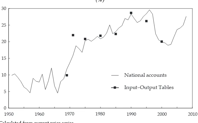
Figure 1 shows that GFCF increased quickly from an average level of 7.5% of GDP until the mid-1960s to about 17% at the start of the 1970s, and then stead-ily but less rapidly to 28% at the onset of the 1997–98 crisis. By 2008 the ratio of
6 For example, where BKE estimated GFCF in 1958 at Rp 8.2 billion (ECAFE 1964: 211), BPS estimated it at Rp 19.8 billion (BPS 1969).
7 Indonesia’s national accounts do not use chain-linking in the estimation of defl ators. 8 The fi rst (1969) I–O Table was published in 1973 (Leknas–Kyodai 1973), but BPS was not formally involved in its creation.
9 The only estimates of public capital formation are for 1981–99 (Everhart and Sumlinski 2003). They suggest a 34% average share of public investment. For 1951–59, BPN/BKE data showed a 32% average share of public investment (Joesoef 1973: 32), but this probably under-estimated private sector investment.
10 The implicit depreciation rate during the years 1960–82 was 6.5%. Neumark (1954) also assumed 5% for 1951–52, while BPN/BKE assumed 3% in the 1950s (Muljatno 1960: 164).
GFCF to GDP had almost recovered from that set-back. The comparison between national accounts data and data from the I–O Tables shows that GFCF may have been under-estimated in the former during the early 1970s. Table 1 confi rms
under-estimation for 1971, 1975 and 1980. Table 2 reveals that according to both sources most GFCF was for structures, machinery and equipment, and transport equipment.
FIGURE 1 Share of Gross Fixed Capital Formation in GDP, 1951–2008a
(%)
B B
B B
B B
B
B
1950 1960 1970 1980 1990 2000 2010
0 5 10 15 20 25 30
National accounts
B Input–Output Tables
a Calculated from current price series.
Sources: Calculated for 1951–57 from Joesoef (1973) and ECAFE (1964); 1958–2008 from the national accounts; 1969, 1971, 1975, 1980, 1985, 1990, 1995 and 2000 from the Input–Output Tables of Indonesia.
TABLE 1 Gross Fixed Capital Formation, 1969–2000
Rp billion % of GDP
Input–Output Tables
National Accounts
Input–Output Tables
National Accounts
1969 270 317 9.9 11.7
1971 937 580 22.0 15.8
1975 2,846 2,572 20.8 20.3
1980 10,550 9,485 21.8 20.9
1985 21,780 22,367 22.3 23.1
1990 59,568 59,758 20.7 28.3
1995 140,245 129,218 26.2 28.4
2000 272,637 275,881 20.0 19.7
Source: BPS, Input–Output Tables of Indonesia, various years; Pendapatan Nasional Indonesia [National Income of Indonesia], various years.
ESTIMATES OF CAPITAL STOCK FOR INDONESIA
Unlike other countries, Indonesia has not conducted a wealth survey on which capital stock estimates could be based.11 The usefulness of wealth surveys in quantitative studies of economic growth can be questioned, because they tend not to correct the value of capital goods for the lower productive capacity of older vintages. Still, the results of such surveys may be useful as a comparator for the results of other approaches, such as the PIM (see, for example,Prados and Rosés 2008: 10–11), particularly when the latter results are based on estimated historical GFCF data.
The BPS estimates of capital formation in constant prices have been used to estimate capital stock. Sundrum (1986: 55, 68) was the fi rst to do so; he used GFCF
and depreciation from the national accounts to extrapolate a rough guess of total
11 Since 1948, the Audit Board (Badan Pemeriksa Keuangan) and its predecessors have estimated the book value of government-owned assets (such as structures, public works, state-owned companies and military assets) in Indonesia (Teulings 1953: 186). However, only the results of the 1949 audit have been published (Ek 1950).
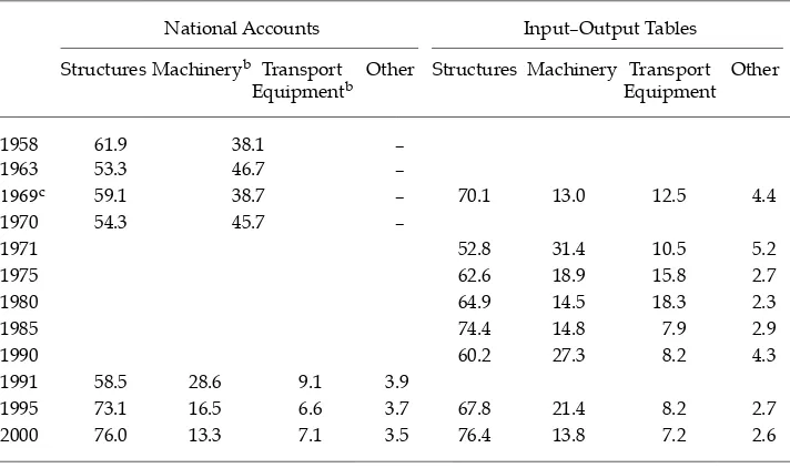
TABLE 2 Share of Four Main Asset Categories in Gross Fixed Capital Formation (GFCF), 1958–2000a
(%)
National Accounts Input–Output Tables
Structures Machineryb Transport
Equipmentb Other Structures Machinery Transport Equipment Other
1958 61.9 38.1 –
1963 53.3 46.7 –
1969c 59.1 38.7 – 70.1 13.0 12.5 4.4
1970 54.3 45.7 –
1971 52.8 31.4 10.5 5.2
1975 62.6 18.9 15.8 2.7
1980 64.9 14.5 18.3 2.3
1985 74.4 14.8 7.9 2.9
1990 60.2 27.3 8.2 4.3
1991 58.5 28.6 9.1 3.9
1995 73.1 16.5 6.6 3.7 67.8 21.4 8.2 2.7
2000 76.0 13.3 7.1 3.5 76.4 13.8 7.2 2.6
a A blank cell indicates that no data (or no disaggregated data) are available for that year. ‘–’ indicates
that the category did not exist for that year. There were no I–O Tables before 1969.
b Data on machinery and transport equipment are combined for 1958–70.
c The 1969 I–O Table gives data at factor cost rather than market prices. GFCF originating from
trans-port, warehousing and trade is therefore excluded.
Sources: National accounts data: 1958: BPS (1969); 1963: Sudirman (1972); 1969: BPS (1970); 1970: Donges, Stecher and Wolter (1973: 212); 1991 and 1995: Saleh (1997: 7–8); 2000: CEIC Asia Database; I–O Tables data: Leknas–Kyodai (1973); BPS, Input–Output Tables of Indonesia.
net capital stock in 1960, in order to generate a net capital stock series for 1960–81 in 1973 prices.
Keuning (1988, 1991) offered an intricate estimation procedure. He estimated GFCF aggregated over three types of capital goods (structures, imported machin-ery and domestically produced machinmachin-ery) between 1953 and 1985, by linking data from the national accounts and other sources and scaling them up to match the 1971 I–O Table and the 1975 and 1980 Social Accounting Matrices. He esti-mated gross value added (GVA) in a similar way for 22 industries during the years 1953–80, and then used the 1980 I–O Table to achieve an allocation of GFCF during the period 1975–85 to those 22 industries. Combining the GFCF and GVA estimates yielded ICVARs for 1975–80, which Keuning then combined with the estimates of GVA in 1980 prices to estimate GFCF in 1980 prices for the 22 indus-tries, disaggregated into three types of capital goods, for 1953–85. He then used these to estimate GFCS for 1975–85 on the basis of a PIM.
While intricate and ingenious, Keuning’s study resulted in COR estimates for the whole economy that were high: 2.2 in 1975, rising to 2.8 in 1985. Extrapolation of Keuning’s GFCS estimates on the basis of total GFCF and depreciation from the national accounts resulted in an implausible COR of over 3.9 by 1999 (Van der Eng 2002: 148–52, 174–5). Even after correction of GDP before 2000 for the degree of under-estimation found in the 2000 revision of Indonesia’s national accounts (Van der Eng 2005), the COR remains implausibly high. Keuning’s methodology may have over-estimated GFCS. His assumption of the productive lives of assets (45 years for construction and 22.5 years for machinery and equipment) may have been too high, and in particular his 1975–85 ICVARs – and therefore his estimates of 1953–85 GFCF and of GFCS – were too high.
As part of their multi-country studies, Nehru and Dhareshwar (1993) and King and Levine (1994) used data on GFCF in Indonesia reported by international agen-cies to construct estimates of capital stock in constant prices using a PIM approach, while others, for example, Collins and Bosworth (1996), have used these estimates to extend the series to later years. None of these studies took account of inconsist-encies and under-estimation in the GFCF data, and their assumptions about the average service life of capital goods were largely arbitrary. The resulting capital stock estimates should therefore be treated with considerable caution.
BPS and BI have made elaborate estimates of capital stock. In an unpublished study, BPS estimated gross and net fi xed capital stock in current and 1993 prices
for 1980–94 (BPS 1996, 1997). The methodology consisted of fi rst disaggregating
GFCF from the national accounts into the relevant categories of capital goods identifi ed in the 1980, 1985 and 1990 I–O Tables; then interpolating these
bench-mark years; and fi nally using a PIM and assumptions about the average service
life of capital goods and the retirement function of these goods to estimate GFCS. However, owing to the very short time span of the GFCF series, the fact that the study did not use an initial capital stock estimate for 1980, and the chosen method of depreciation, the implicit rate of depreciation in the BPS study was too high for 1981 and too low for 1994, and the results were not usable.12
12 BPS (2007) uses the same methodology, but with new estimates of asset lives (see table 4) to extend the capital stock estimates to 2000.
Sigit (2004: 101–3, 124–5) considered this BPS report for his study of total factor productivity growth in Indonesia, but decided against using it. He used existing GFCF series for 1960–2000, corrected for inconsistencies and under-estimation, to estimate total GFCS in 1993 prices for 1975–2000 on the basis of a PIM. He assumed a short average service life of productive assets of 15 years and a rate of depreciation of 3%. Sigit then allocated GFCS for 1980–94 to nine economic sectors on the basis of the BPS (1996) fi gures, extrapolating 1995–2000
on the basis of regressions. The resulting sectoral estimates of GFCS are neces-sarily crude.
A research team at BI estimated gross and net fi xed capital stock in 1993 prices
for 1960–2002 (Wicaksono, Ariantoro and Sari 2002; Wicaksono and Ariantoro 2003; Yudanto et al. 2005). It used a similar approach to that of BPS, but included results from the 1995 and 2000 I–O Tables. The team interpolated between the GFCF benchmark years from the I–O Tables to obtain a new time series of GFCF for 29 capital goods during the years 1980–2000. It then apportioned GFCF to nine categories of capital goods and to 10 economic sectors on the basis of the I–O Tables, to generate disaggregated GFCF data in current prices. The current price series were combined with assumptions about the average life of nine capi-tal goods and about their retirement, in order to produce estimates of capicapi-tal stock in current prices. Wholesale price indices for the nine goods categories were then used for defl ation and the creation of series in constant 1993 prices. As the longest
life span of assets was assumed to be only 20 years (for buildings), the fi rst
‘com-plete’ estimate of capital stock was for 1999. This estimate was extrapolated on the basis of what the BI team labelled a ‘gross-up’ method (see item 3 below), fi rst for
1980–98 and then for 1960–79.
These BI estimates offer a viable methodology, although they contain some shortcomings, including the following:
1 Saleh (1997: 4) noted that the BPS estimates of GFCF are incomplete, as they cover only the acquisition of domestically produced new capital goods and new and used imported capital goods (all estimated on the basis of the commodity fl ow
method). They therefore exclude investment in cultivated assets, particularly in agriculture, such as perennial crops and livestock.13 They also exclude new investment for the improvement of existing assets (such as roads and other existing infrastructure). Nor is the disposal of capital goods through exports (for example, ships and aeroplanes) accounted for. Another problem is that the use of various materials in the construction industry, such as steel and electrical equipment, is not fully accounted for (Rachman 2004: 2, 4).
2 The choice of 1980 as the starting point for the study ignores information available from the 1971 and 1975 I–O Tables.
13 Hooley (1967: 202) noted this as a serious omission in GFCS estimates in less developed countries. The coverage of investment in livestock is incomplete in Indonesia’s I–O Tables and non-existent in the national accounts. Investment in perennials is not covered in either source. A major prerequisite for the analysis of long-term economic growth in Indonesia is the estimation of capital formation and capital stock in agriculture, given the prominence of agricultural output in the economy until the 1970s. Possible methodologies are outlined in Shukla (1965) and Nomura (2006).
3 The ‘gross-up’ method and the methods used to allocate GFCF to types of capital goods and to economic sectors are not unambiguously explained and are therefore not immediately replicable.
4 Estimates of average asset lives were obtained from BPS, which in turn obtained them from Decrees of the Minister of Finance (KMK [Keputusan Menteri Keuangan] 961/1983 and 826/1984 on Taxation) containing allowable rates of depreciation for accounting purposes for broad asset groups (BPS 1996: 3, 5; BPS 1997: 3).14 The experience of other countries has indicated that tax offi ce
estimates of depreciation do not always resemble actual asset lives (see, for example, Lützel 1977: 69; Blades 1983: 5; OECD 2001: 47–8). Indonesia is not likely to be an exception. For example, the Indonesian taxation rules allow companies in capital-intensive industries to employ accelerated depreciation rates relative to other countries (Gordon 1998: 25). Indeed the average asset lives used by BPS and BI are very short compared with those of other countries (see, for example, Blades 1993). Consequently, both may have under-estimated capital stock.
While it cannot take account of the fi rst point, this article will address the issues
raised under points 2, 3 and 4 in the next section.
NEW ESTIMATES OF CAPITAL FORMATION AND CAPITAL STOCK
This article will now present new estimates of GFCF in 2000 prices for the period 1951–2008, which will be apportioned to 28 types of capital goods on the basis of the I–O Tables. Assumptions about asset lives and a simple PIM will then be used to aggregate the GFCF data and estimate GFCS. Unfortunately it is not possible also to apportion GFCF to key sectors. While the published I–O Tables specify the economic sector delivering each type of capital good, they do not identify the economic sector for which the capital goods are destined. Unlike Keuning (1988, 1991), BPS (1996, 2007) and Yudanto et al. (2005), the author did not have access to the unpublished I–O data that would have identifi ed the
destination.
14 The Indonesian government simplifi ed its tax system in 1984 (making further changes in 1995 and 2000). Law 7/1983 gave depreciation rates for buildings and four other asset groups by useful life (Uppal 2003: 20–1, 157–8). Further regulations (for example, 961/ KMK.04/1983) interpreted these rules. The latest regulation, 138/KMK.03/2002, speci-fi ed a range of specifi c assets in each of these four groups. Neither the accounting stand-ards issued by the Indonesian Institute of Accountants (Pernyataan Standar Akuntansi Keuangan, PSAK), particularly No. 46, Standar Akuntansi Pajak Penghasilan (on in-come taxes), nor the Indonesian government accounting standards (Pernyataan Standar Akuntansi Pemerintahan, PSAP), particularly No. 07 Tentang Akun tansi Aset Tetap (on accounting of fi xed assets), proposes depreciation rates for specifi c types of assets. The fi rst set of standards has no legal grounding, so there is no legal obligation on companies to follow them. However, a cursory check of the fi nancial statements of some major public companies in Indonesia suggests that they follow the depreciation rates set out in the tax regulations.
Re-estimating gross fi xed capital formation, 1951–2008 The following steps were taken to re-estimate GFCF:
(a) Creation of a single GFCF price index by linking the implicit defl ators of GFCF
from the national accounts for 1951–58, 1958–71, 1971–83, 1983–88, 1988–2000 and 2000–08 to form a new continuous price index for the period 1951–2008, in which 2000 = 100.
(b) Interpolation of total GFCF from data for the benchmark years of 1971, 1975, 1980, 1985, 1990, 1995 and 2000 in the I–O Tables, using growth rates of GFCF in current prices from the national accounts, in order to correct for the under-estimation of GFCF in the national accounts, particularly in 1971, 1975 and 1980, demonstrated in table 1.15 This yields a new time series of total GFCF for 1971–2000 in current prices.
(c) Defl ation of total GFCF using the GFCF price index from step (a) to form a new
time series of total GFCF for 1971–2000 in 2000 prices.
(d) Extrapolation of total GFCF in 2000 prices for 1951–70, using growth rates of GFCF in constant prices from the national accounts for 1958–71 and from Joesoef (1973: 32) for 1951–58 to create a series of total GFCF for 1951–2000 in constant 2000 prices.
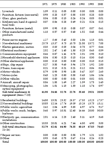
(e) Apportionment of GFCF to 28 categories of capital goods for 1971–2000 using the interpolated shares shown in table 3 for the benchmark years of the I–O Tables and GFCF from step (d). Table 3 shows that most GFCF was in structures, the share of which increased from 53% in 1971 to 76% in 2000, to the detriment of the share of machinery and equipment, which decreased from 42% to 21%. (f) Extrapolation for 1958–70 of the total of categories 7–20 and 21–26 in table 3 on
the basis of GFCF in 1960 prices in ‘construction and works’ and ‘machinery and equipment’ from BPS (1969), Sudirman (1972), BPS (1970) and Donges, Stecher and Wolter (1973: 212). Deduction of these two groups from the GFCF series for 1958–70 from step (d) created a group ‘other’, which comprises items 1–6, 27 and 28 shown in table 3. The results were then allocated to individual categories in these three groups, on the basis of their 1971 shares shown in table 3.
(g) Extrapolation of 1951–57 GFCF from (d) using 1958 shares of the 28 categories from step (f).
(h) Extrapolation of 2000–08 GFCF in the four asset groups shown in table 2 from the CEIC Asia Database, apportioned to the 28 sub-categories within the four groups on the basis of their 2000 shares in table 3.
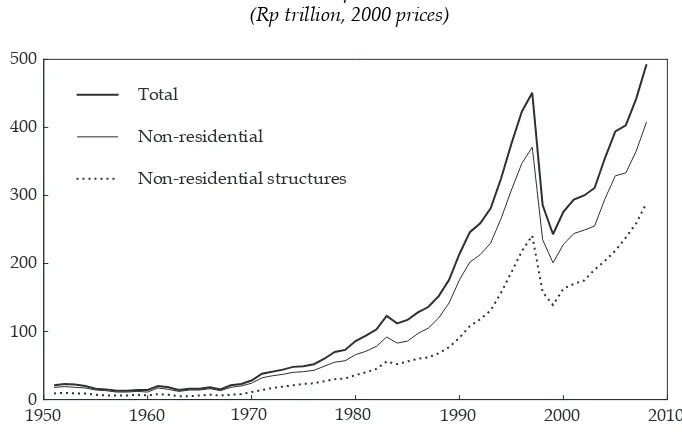
The results are summarised in fi gure 2, which shows that GFCF quadrupled
between the 1960s and the 1980s, and then quadrupled again to the mid-1990s. The 1997–98 crisis and its aftermath caused a considerable fall in GFCF, although the trough in 1999 was still at a level comparable to 1991. GFCF recov-ered to 1997 levels in 2007. The chart also indicates that the trend was largely driven by non-residential capital stock, particularly non-residential structures.
15 The 1969 I–O Table was not used, because it did not offer a comparable breakdown of GFCF.
TABLE 3 Shares of Capital Goods in Gross Fixed Capital Formation, 1971–2000a
(%)
1971 1975 1980 1985 1990 1995 2000
1 Livestock 1.09 0.11 0.03 0.00 0.00 0.08 0.08 2 Furniture, fi xtures (non-metal) 0.93 0.28 0.37 0.38 0.35 0.28 0.03 3 Glass, glass products 0.04 0.08 0.13 0.26 0.24 0.03 0.01 4 Kitchenware, hand &
agricul-tural tools
0.07 0.06 0.28 0.49 0.21 0.24 0.15
5 Furniture, fi xtures (metal) 0.99 0.98 0.18 0.08 0.07 0.07 0.61 6 Other manufactured metal
products
1.18 0.57 0.57 0.43 1.52 0.48 0.44
7 Prime mover engines 1.27 0.66 0.48 0.53 1.06 1.13 0.81 8 Non-electrical machinery 25.79 13.37 9.73 10.70 21.58 13.72 7.08 9 Electric generators, motors 0.08 0.08 0.05 0.04 0.78 0.77 0.66 10 Electrical machinery 2.52 2.47 1.45 1.30 0.25 0.63 0.59 11 Communications equipment 0.66 0.87 1.41 0.78 2.31 2.98 3.10 12 Household electrical appliances 0.04 0.30 0.25 0.15 0.16 0.30 0.45 13 Other electrical appliances 0.00 0.15 0.00 0.00 0.00 0.10 0.13 14 Ships, ship repair 0.27 3.58 9.63 3.96 2.73 1.92 2.00 15 Trains, train repair 0.21 0.13 0.21 0.21 0.12 0.06 0.03 16 Motor vehicles 8.79 8.93 5.93 1.08 3.47 3.37 2.63 17 Motor cycles 0.43 1.23 0.80 0.38 0.43 1.06 1.04 18 Other vehicles 0.00 0.00 0.00 0.01 0.03 0.02 0.01 19 Aircraft, aircraft repair 0.86 1.88 1.69 2.27 1.39 1.73 1.45 20 Measuring, photographic,
optical equipment
1.06 1.01 1.13 1.33 1.18 1.74 0.97
Sub-total machinery & equipment (items 7–20)
41.98 34.66 32.76 22.76 35.48 29.51 20.95
21 Residential buildings 14.80 15.51 23.52 26.37 17.58 18.23 17.37 22 Non-residential buildings 10.85 12.14 17.74 19.89 13.26 13.75 13.11 23 Public works: agriculture 2.62 2.84 4.89 5.85 4.97 6.76 9.17 24 Public works: roads, bridges,
harbours
3.68 5.97 10.31 12.40 16.46 20.00 30.03
25 Electricity, gas, communication installations
2.51 6.14 2.23 2.40 3.11 4.19 3.68
26 Other construction 18.33 20.01 6.21 7.44 4.80 4.90 3.08
Sub-total structures (items 21–26)
52.79 62.61 64.90 74.35 60.19 67.83 76.43
27 Repair services 0.00 0.00 0.00 0.58 1.79 1.21 1.02 28 Other 0.93 0.63 0.78 0.67 0.14 0.26 0.28
Total 100.00 100.00 100.00 100.00 100.00 100.00 100.00
a The 1969 I–O Table does not offer a comparable disaggregation of GFCF and is excluded. Categories
7–9 for 1971–85 (italicised) are estimated on the basis of 1990 proportions of ‘non-electrical machinery’; categories 21–22 for 1980–2000 (italicised) are estimated on the basis of 1971–75 average proportions of ‘residential and non-residential buildings’.
Source: BPS, Input–Output Tables of Indonesia.
Estimating gross fi xed capital stock, 1950–2008
The estimates of GFCF are used to estimate capital stock on the basis of a PIM, as recommended in the UN’s 1993 System of National Accounts. This can take the form of gross fi xed capital stock (GFCS or KG) or net fi xed capital stock (KN) in constant
prices, as shown in equations 2 and 3.
KtG KtG It Rt ItGj r j
The difference between the two lies in the disaggregation of depreciation in the net fi xed capital stock equation (3) into (a) foreseen obsolescence, or the retirement
of capital goods (R) over their service life (L), so that only a proportion remains of each vintage (j) of a capital good in a given year; and (b) depreciation in its con-ventional sense for accounting purposes, that is, the annual loss of value of capital stock due to wear and tear on, or aging of, capital goods, refl ecting the decline in
the relative effi ciency of each vintage of a capital good as it ages (V). The terms r(j)
and v(j) are the retirement function and the depreciation function, respectively. To analyse economic growth, KG is the most appropriate concept to use, if we
assume that repair and maintenance compensate for wear and tear until the end of the service life of a capital good. It is arguably less appropriate for this purpose to estimate KN and account for the decline of asset effi ciency with age. KN is a
use-ful concept for the purpose of surveying a country’s national wealth, as it takes account of the age composition of different categories of capital goods. It is cer-tainly appropriate for company and tax accounting purposes, where depreciation
FIGURE 2 Gross Fixed Capital Formation, 1951–2008a
(Rp trillion, 2000 prices)
19500 1960 1970 1980 1990 2000 2010 100
Sources: See text and Van der Eng (2008a).
records the loss of the value of assets used for production purposes, to approxi-mate the ‘fair value’ of assets. However, when depreciation is assessed as being faster (for instance, for reasons of taxation) than the actual effi ciency decline of
capital goods, the net fi xed capital concept is likely to under-state the capital stock
actually employed for production purposes. There is no reliable evidence of the rate of effi ciency decline of capital goods, and the rates of depreciation used for
accounting and taxation purposes in Indonesia seem high relative to those used in other countries, as indicated in the previous section.
To estimate KG, or GFCS, we need indications of the average service life of the
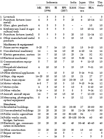
various categories of capital goods, and we must choose an appropriate retirement function. Table 4 summarises the available information on average asset lives in Indonesia. As noted in the previous section, the asset lives used in the BPS (1996) and BI studies are based largely on taxation data. To indicate that these estimates may be rather low, estimates of the service life of assets used in the calculation of capital stock in India, Japan and the USA are included in table 4. The 20-year life assumed for structures in Indonesia seems particularly low, which explains why BPS (2007) assumed higher asset lives for some categories.
Estimates of asset service lives differ considerably across countries (Blades 1983: 12–15; 1993: 13–16). Such differences seriously impair inter-country com-parisons of capital stock, as Maddison (1995) argued; this led him to re-estimate capital stock in several countries using USA-based standardised asset lives of 39 years for ‘non-residential structures’ and 14 years for ‘machinery and equip-ment’. The choice of standardised asset lives may in principle facilitate com-parison, but where different asset life estimates across countries refl ect actual
observation of these asset lives, standardised asset lives would introduce an ele-ment of arbitrariness.
There are no historical data on the lives of productive assets in Indonesia.16 To accommodate the 28 asset categories, this study uses the average asset lives shown in the last column of table 4, which are based particularly on asset lives identifi ed in the more detailed studies for the USA, Japan and India. The asset
lives used here are generally higher than those used in the BPS (1996) and BI stud-ies, and for structures they resemble the asset lives used in BPS (2007). It is pos-sible to assume that the average service life of particular categories of productive assets in Indonesia changed over time. They may have decreased, as has been the experience for other countries (Blades 1983: 16; Blades 1993: 25–30; OECD 2001: 50–1). Indeed, casual impressions may suggest that public structures in Indonesia such as railway stations and irrigation structures built in the past may have lasted longer than those built in recent decades, although that also depends crucially on whether regular maintenance work was carried out. However, there is no way to generalise such impressions.
Little is known about the actual retirement of capital goods by companies in Indonesia during their service life. Several possible retirement patterns can be assumed. One is the ‘one-hoss shay’ or simultaneous exit method, whereby a capital good delivers the same services for each vintage and is scrapped at the end of its service life. While anecdotal evidence may suggest that capital goods
16 As part of its re-kindled work on estimating capital stock, BPS started a fi rst survey into asset lives on a limited scale in 2008. The results are not yet available.
TABLE 4 Average Service Lives of Productive Assets: Indonesia, India, Japan and USA 8 Non-electrical machinery 16 – 16 10 20 6–10 16 16 9 Electric generators, motors 16 7 18 15 25 26 32 32 10 Electrical machinery 16 – 18 10 15 9–30 16 16 11 Communications
equip-ment 8 7 10 7 15 9 11–15 13
12 Household electrical
appliances 4 10 10 5 15 19 9–11 10
13 Other electrical appliances 4 – 10 5 15 5–16 9–11 10 14 Ships, ship repair 16–20 10 10 15 15 21 27 27 15 Trains, train repair 20 10 10 20 20–33 15 28 28 16 Motor vehicles 4–8 7 10 5 10 9–15 9–14 12
17 Motor cycles 4 3 10 5 10 5 8–10 10
18 Other vehicles 8–16 – 10 5 8 5 9–14 12 19 Aircraft, aircraft repair 16 7 10 15 10 7 12–20 12 20 Measuring, photographic,
optical equipment 8 6 5 6 15 12 10 10
Structures
21 Residential buildings 20 20 20 20 20–80 27 20–80 30 22 Non-residential buildings 20 20 20 20 80 21–26 30–50 30 23 Public works: agriculture 20 20 20 20 30–100 36 – 20 24 Public works: roads,
bridges, harbours 20 20 20 40 55–100 50–56 60 40 25 Electricity, gas,
communi-cation installations 20 20 20 40 45 38–40 40–45 40 26 Other construction 20 20 20 20 35 13 60 40
27 Repair services – – 16 5 – – – 5
28 Other – – 16 5 – – 5 5
a MK, BPS, BI, K&M, Nomura and BEA refer to the sources (see below). None of the sources identifi ed
each of the 28 categories of capital goods explicitly. The service lives reported in the sources have been broadly applied to the 28 categories. ‘–’ indicates that the study had no estimates for that category. Sources: MK: Ministry of Finance of Indonesia, Keputusan Menteri Keuangan (Decree of the Minister of Finance) No. 138/KMK.03/2002, <http://kanwilpajakkhusus.depkeu.go.id/penyuluhan/pph/gol-harta.htm>; BPS (1996: 5); BI: Yudanto et al. (2005: 187); BPS (2007: 26–7); K&M: Kulshreshtha and Malhotra (1998: 14); Nomura: Nomura (2005a: 37; 2005b: 21); BEA: BEA (2003).
have been kept productive for long periods in Indonesia, it is unlikely that this would have applied to all capital goods or all vintages. It is more appropriate to assume a rate of retirement. Different patterns can be assumed, such as linear retirement, which reduces the stock of a vintage of a capital good by the same amount each year, or geometric retirement, which reduces the stock of a vintage of a capital good at the same rate each year, until the last remaining vintage is at the end of its service life (Blades 1983: 17–21; Blades 1993: 18–20; OECD 2001: 53–8). Comparisons of the different methods of retirement indicate that – except for the simultaneous exit pattern – GFCS estimates are relatively insensitive to the retirement pattern used (Blades 1983: 27; O’Mahony 1996; Yudanto et al. 2005: 186–7). For the sake of simplicity, we use a linear retirement function r(j) as shown in equation 4 for all capital goods in an asset category. This implies that equal amounts of the value of a capital stock of a given vintage are deducted from the capital stock for every year until the maximum service life of the asset has been reached.
r j L j L
( )=( − ) where 0≤ ≤j L (4)
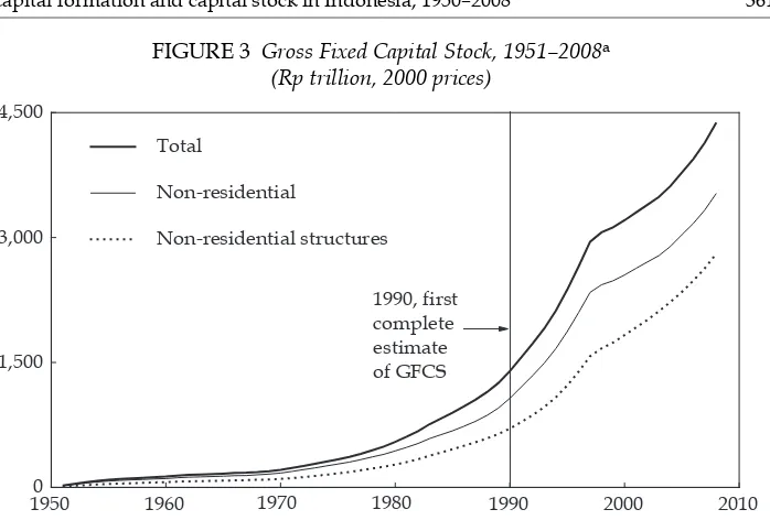
The disaggregated annual estimates of GFCF, combined with average asset lives and the method of depreciation used for national accounting purposes, allow the estimation of GFCS on the basis of a PIM. The results are summarised in fi gure 3. As the longest life span of our asset categories is 40 years (table 4),
the fi rst ‘complete’ estimates of GFCS are for 1990. The chart shows that between
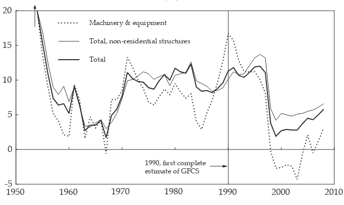
1990 and 1997 GFCS doubled, before the rate of growth slowed following the 1997–98 crisis. The chart also indicates that the trend was driven largely by non-residential capital stock, particularly non-non-residential structures, as suggested in fi gure 2. Figure 4 confi rms these impressions. During the period 1971–97,
growth of total GFCS was 10% per year on average, broadly in line with the FIGURE 3 Gross Fixed Capital Stock, 1951–2008a
(Rp trillion, 2000 prices)
19500 1960 1970 1980 1990 2000 2010 1,500
3,000 4,500
Total
Non-residential
Non-residential structures
1990, first complete estimate of GFCS
Sources: See text.
trend in the category non-residential structures, rather than with that in machin-ery and equipment.
Figure 5 shows the implicit rate of depreciation, as a percentage of GDP, result-ing from the retirement of productive assets durresult-ing their service life. Clearly, the total rate of depreciation after 1990 far exceeds the implicit 5% rate of depreciation
FIGURE 5 Implicit Rate of Depreciation of Capital Stock, 1951–2008 (% of GDP)
19500 1960 1970 1980 1990 2000 2010 3
6 9 12 15
Total as % of GDP
Non-residential total
Machinery & equipment
Total (BPN/BPS rate)
1990, first complete estimate of GFCS
Sources: Implicit BPN/BKE rate (see footnote 5) 1951–59 from Joesoef (1973: 32); implicit BPS rate from the national accounts; other implicit rates are results of this study (see Van der Eng (2008a). They are expressed as a ratio of GDP estimates for 1951–2008 (in 2000 prices) from Van der Eng (2008b), updated to 2008.
FIGURE 4 Annual Growth of Gross Fixed Capital Stock, 1952–2008 (%)
1950 1960 1970 1980 1990 2000 2010 -5
0 5 10 15 20
Total
Total, non-residential structures Machinery & equipment
1990, first complete estimate of GFCS
Sources: See text and Van der Eng (2008a).
in the national accounts during the years 1983–2008. Most of the depreciation is driven by non-residential capital stock, comprising both non-residential structures and machinery and equipment. The rate of depreciation was probably higher than the 5% of GDP assumed by BPS. In the absence of detailed capital stock data, BPS measured the depreciation of fi xed capital stock on the basis of an assumed rate,
as was done in other countries. However, advances in the measurement of capital stock have led to better substantiated estimates that often exceed the previously assumed rates. Consequently, the national accounts of developed countries now estimate the consumption of fi xed capital stock on the basis of capital stock
esti-mates that are PIM-based. For example, in Australia the consumption of fi xed
capital stock is now estimated to be 15–16% of GDP (ABS 2007) and in the USA no less than 16–20% of GDP (BEA 2008).
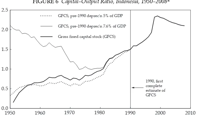
Figure 6 shows the COR for 1950–2008 that is a consequence of the calculations outlined above, as well as two CORs that are the result of the backward extrapola-tion of total GFCS from 1990 on the basis of GFCF and two assumpextrapola-tions about the rate of retirement of productive assets (5%, which is the 1983–2008 implicit rate in the national accounts, and 7.6%, which approximates the 1990 implicit deprecia-tion rate) according to equadeprecia-tion 5.
K K I Y
t G
t G
t t
−1= − +ρ (5)
where KG = GFCS, I = GFCF, ρ = rate of depreciation (or rather, of retirement of
productive assets) as a percentage of GDP, and Y = GDP (all in constant prices). Figure 6 shows that the COR based on the assumption that ρ = 5% follows the COR based on GFCS estimated above, which we know is incomplete until 1990. Hence, the COR based on the assumption that ρ = 7.6% is likely to be more real-istic. It shows a gradual decline between 1950 and 1967, which refl ects the fact
FIGURE 6 Capital–Output Ratio, Indonesia, 1950–2008a
1950 1960 1970 1980 1990 2000 2010 0.0
0.5 1.0 1.5 2.0 2.5
Gross fixed capital stock (GFCS) GFCS, pre-1990 deprec'n 7.6% of GDP GFCS, pre-1990 deprec'n 5% of GDP
1990, first complete estimate of GFCS
a The three series show the ratio of GFCS to GDP, with GFCS estimated in three ways, as shown in
the legend.
Sources: See text and Van der Eng (2008a).
that the growth of GDP was low, at 2.8% per year, and GFCF modest. This was followed by a rapid decline during the years 1967–73 and stagnation from 1973 to 1981, a period when economic growth accelerated to 7.8% per year, higher than the growth of GFCF. Between 1981 and 1997, the COR increased quickly, from 1.0 in 1981 to 1.9 in 1997 as the growth of GFCF outpaced that of GDP. The COR jumped to 2.3 in 1999 owing to the fall in GDP during the 1997–98 crisis.
The increase in the COR since 1981 may be a consequence of accelerated struc-tural change away from agriculture towards greater economic dependence on production, income and employment in more capital-intensive exploits, particu-larly manufacturing. The share of agriculture in total GDP in current prices, with presumably a lower COR than that in the industrial sector, decreased continu-ously from an average of 35% in the 1960s to 12% in 1997. Meanwhile, the share of industrial production increased from a low 15% during the 1960s to 40% in 1997, suggesting that new investment in manufacturing is likely to have contributed to the COR’s rise. Particularly during the 1990s, the share of investment in non-residential structures (items 22–26 in table 3) increased quickly from 43% in 1990 to 50% in 1995 and 59% in 2000.
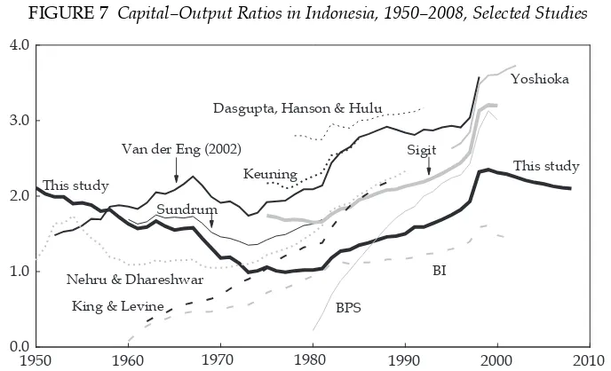
Figure 7 compares the CORs estimated in this article with COR estimates for Indonesia from other studies. All trends are of similar proportions to our esti-mates, apart from the very low levels in the BPS (2007) estimates for the early 1980s, which are due to the ‘build-up’ of aggregated GFCF from the fi rst
‘instal-ment’ in 1980. The BI estimates are signifi cantly lower than ours, owing largely
to the shorter asset lives used in the BI study (table 4), particularly for structures. FIGURE 7 Capital–Output Ratios in Indonesia, 1950–2008, Selected Studies
1950 1960 1970 1980 1990 2000 2010 0.0
1.0 2.0 3.0 4.0
This study Keuning
Van der Eng (2002)
Dasgupta, Hanson & Hulu
Yoshioka
Sigit
Sundrum
Nehru & Dhareshwar
King & Levine BPS
BI
This study
Sources: Sundrum (1986), 1973 prices; Keuning (1988, 1991), 1980 prices; BI, Yudanto et al. (2005), 1993 prices; BPS (2007), 1993 prices ‘delayed survival’ method; Nehru and Dhareshwar (1993), 1987 prices; King and Levine (1994), 1985 prices; Van der Eng (2002), 1983 prices; Yoshioka (2002), current prices; Sigit (2004), 1993 prices; Dasgupta, Hanson and Hulu (2002), 1983 prices. All capital stock estimates are expressed as a ratio of GDP as given in these sources or from the national accounts, except that capital stock estimated in this study is expressed as a ratio of GDP estimates for 1950–2008 (in 2000 prices) from Van der Eng (2008b, updated to 2008).
The estimates of Dasgupta, Hanson and Hulu (2002) and Yoshioka (2002) seem unrealistically high, while the discrepancies between our estimates and those of Sundrum (1986), Keuning (1988, 1991) – and by implication Van der Eng (2002) – and Sigit (2004) are due to the differences in methodologies outlined above. The signifi cant differences between our estimates and those of Nehru and Dhareshwar
(1993) and King and Levine (1994) are diffi cult to explain in the absence of detailed
information about data sources and estimation procedures for Indonesia in these studies. But the signifi cantly different trends in the CORs clearly suggest that
cau-tion is appropriate when using the capital stock data from the latter two studies, at least for Indonesia.
How plausible are the COR estimates in fi gure 7? A plausibility check can be
made through comparison with COR estimates of countries at a similar level of development. Snodgrass (1966: 68, 75) estimated the COR for Malaya to be 1.4–1.7 in 1954 and 1.8–1.9 in 1963. Chou (1966: 73) suggested a COR of 2 for Malaya (including Singapore) in the early 1950s, while Abraham and Gill (1969: 52) esti-mated an average COR of 1.45 in 1960–66 for West Malaysia. These estimates are all broadly comparable with this study’s estimates, as shown in fi gures 6 and 7.
A major problem with COR estimates for different countries is that their data on capital formation and capital stock are based on different defi nitions and
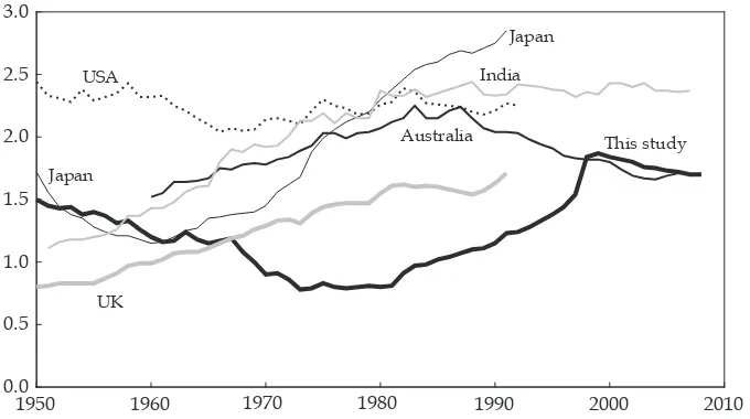
meth-ods of calculation. Maddison (1995) offered estimates of GFCS based on aver-age asset lives that are to an extent comparable with the averaver-ages used in this article (generally 30–40 years for structures and 10–16 years for machinery and equipment). Figure 8 compares our estimates of the non-residential COR with those of Maddison (1995) for Japan, the UK and the USA, and with data for India and Australia, which also used comparable asset lives. Figure 8 suggests that our
FIGURE 8 Non-Residential Capital-Output Ratios, 1950–2008, Selected Countries
1950 1960 1970 1980 1990 2000 2010 0.0
0.5 1.0 1.5 2.0 2.5 3.0
USA
Japan
UK Japan
This study Australia
India
Sources: USA, Japan, UK capital stock: Maddison (1995: 149–56); GDP: Maddison (2003) in 1990 Geary– Khamis dollars; Australia: ABS (2007) in current prices; India: CSO (2007, 2008) in 1999–2000 prices; non-residential capital stock in 2000 prices are from this study, assuming a pre-1990 depreciation rates of 6.1% of GDP (Van der Eng 2008a, updated to 2008), expressed as a ratio of GDP for 1950–2008 in 2000 prices from Van der Eng (2008b, updated to 2008).
estimates of capital stock in Indonesia relative to GDP were comparable with those for other countries in the 1950s, particularly Japan and India. Our COR estimate was around 0.8 in the 1970s, which is quite low in international terms. It increased during the 1980s and 1990s to more comparable levels internationally, suggesting that our estimates of GFCS are not too low for the 1990s.
Even so, Indonesia is still a less developed country, where the contribution of manufac turing industry to GDP has increased, but where a large part of that sec-tor is still labour- rather than capital-intensive, and where agriculture and serv-ices, with their low CORs, are still signifi cant. Consequently, our estimates of
Indonesia’s COR in 1998–99 of 2.3 to 2.4 for total GFCS in fi gure 7 and 1.8 to 1.9 for
non-residential GFCS in fi gure 8 appear to be high, even though the 1998–99 spike
in both CORs was a consequence not of a sudden increase in GFCS, but rather of a signifi cant fall in GDP during the crisis years. The high COR in 1998–99 suggests
considerable under-utilisation of productive capacity, particularly in the form of structures as opposed to machinery and equipment.
Figures 7 and 8 reveal that Indonesia’s COR increased signifi cantly from 1980
onward, rather as India’s did between 1950 and 1980, Australia’s from 1960 to 1983, Japan’s from 1960 to 1991 and the UK’s from 1955 to 1982, but in sharp contrast with that of the USA between 1950 and 1991. It is surprising to fi nd such
a signifi cant increase at a still early stage in Indonesia’s economic development
process. During this stage there should still be signifi cant opportunities to absorb
technology and improve productivity in order to sustain economic growth, rather than relying increasingly on the mobilisation of investment capital for this pur-pose. Kosai (2005) discusses this phenomenon in the case of Japan, arguing that Japan left the growth trajectory led by technological development and produc-tivity growth in the 1970s in favour of growth led by capital mobilisation. This process continued during the 1990s, with Japan reaching a COR of 4.0 in 2003, compared with 2.3 in the USA and 1.7 in the UK (Maddison 2007: 305, 385). While capital accumulation in Indonesia appears to have followed a similar path to that of Japan during the early 1990s, that development clearly came to an end in 1998. During the 1997–98 crisis GFCF contracted substantially, implying that producers chose to look for ways to enhance the productive use of existing capital goods (Ishihara and Marks 2005) rather than seek fi nance for new investments.
CONCLUSION
The research into the estimation of capital stock at BPS and Bank Indonesia sig-nifi cantly advanced the debate about the measurement of the country’s capital
stock and the possibility of a better informed discussion about long-term growth and structural change in Indonesia. As noted above, not all aspects of the meth-odology in the BI study are clear, while some aspects could be re-considered. This article has drawn attention to the fact that BI opted to use 1980 as the starting point for its estimation, thus ignoring earlier information on GFCF in Indonesia and estimating capital stock with assumed asset lives that may be too low.
This article has highlighted these issues and used historical data on GFCF to estimate GFCS from 1951. It may be obvious that more work on estimating GFCF and GFCS in Indonesia can be done. First, for historical estimates of GFCF, the methods used for estimating GFCF at BPS in the past need to be revisited, made
consistent where possible and augmented where necessary in order to re-estimate GFCF back in time. Second, the sensitivity of the estimates of GFCS to different assumptions about the service life of capital goods needs to be assessed, possibly on the basis of alternative information on asset lives in Indonesia if it exists.
Despite these shortcomings, the article has indicated that the levels of GFCF in Indonesia during the 1980s and 1990s had no precedent, and they sustained a rapid increase in the country’s GFCS. The ratio of capital stock to GDP indicates that the increase in CFCS during the period 1990–97 was very substantial. Further research could explore whether capital accumulation contributed to the excess productive capacity that exacerbated the country’s economic woes during and after the 1997–98 crisis. Since 1999, Indonesia has sustained modest but signifi cant
rates of growth despite low levels of GFCF growth (Van der Eng 2004: 3). Such low levels of investment have increased the utilisation of existing productive capac-ity (Ishihara and Marks 2005). GFCF returned to pre-crisis levels in 2007, but the COR decreased. In combination with sustained economic growth, this suggests an improvement in the productive use of available capital goods.
REFERENCES
Abbas, Saiyid Asghar (1955) Capital Requirements for the Development of South and South-East Asia, Wolters, Groningen.
Abraham, William Israel (1958) ‘Investment estimates of underdeveloped countries: an appraisal’, Journal of the American Statistical Association 53: 66–79.
Abraham, William Israel (1967) ‘Statistics and national planning, some comments’, Philippine Economic Journal 6: 90–4.
Abraham, William Israel and Gill, Mahinder Singh (1969) ‘The growth and composition of Malaysia’s capital stock’, Malayan Economic Review 14 (2): 44–54.
ABS (Australian Bureau of Statistics) (2007) Australian System of National Accounts, 2006–07 (cat. no. 5204.0), ABS, Canberra, available at <http://www.abs.gov.au>.
BEA (Bureau of Economic Analysis) (2003) Fixed Assets and Consumer Durable Goods in the United States, 1929–99, BEA, US Department of Commerce, Washington DC.
BEA (Bureau of Economic Analysis) (2008) National Economic Accounts, BEA, US Depart-ment of Commerce, Washington DC, available at <http://www.bea.gov/national/ index.htm>.
Blades, Derek (1983) ‘Service lives of fi xed assets’, OECD Economics and Statistics Depart-ment Working Paper No. 4, Organisation for Economic Co-operation and Develop-ment, Paris.
Blades, Derek (1993) ‘Methods used by OECD countries to measure stocks of fi xed capital’, OECD National Accounts Sources and Methods No. 2, Organisation for Economic Co-operation and Development, Paris.
BPN (Biro Perancang Negara, State Planning Bureau) (1957) ‘Model pembangunan ekonomi dalam Indonesia [A study of the Indonesian economic development scheme]’, Ekonomi dan Keuangan Indonesia [Indonesian Economics and Finance] 10 (8): 483–526 (English translation published in Ekonomi dan Keuangan Indonesia 10 (9): 600–42).
BPS (Biro Pusat Statistik, Central Bureau of Statistics) (1969) Gross domestic fi xed capital formation by type of capital goods at 1960 prices, 1958–1968, Unpublished note, BPS, Jakarta (available in the Indonesia Project library, Australian National University, Can-berra).
BPS (Biro Pusat Statistik, Central Bureau of Statistics) (1970) Pendapatan Nasional Indonesia 1960–1968 [National Income of Indonesia 1960–1968], BPS, Jakarta.