11 (2001) 139 – 163
The day-of-the-week regularity in the stock
markets of China
Gongmeng Chen
a,*, Chuck C.Y. Kwok
b, Oliver M. Rui
caThe Department of Accountancy,The Hong Kong Polytechnic Uni
6ersity,Hung Hom, Kowloon,Hong Kong
bDepartment of International Business,Uni
6ersity of South Carolina,Columbia,SC29208,USA cThe Department of Accountancy,The Hong Kong Polytechnic Uni
6ersity,Hung Hom, Kowloon,Hong Kong
Received 21 July 1999; accepted 11 March 2000
Abstract
This paper examines the day-of-the-week effect in the stock markets of China. We find negative returns on Tuesday after January 1, 1995. This Tuesday anomaly disappears after taking the non-normality distribution and spillover from other countries into account. The finding suggests that this day-of-the-week regularity in China may be due to the spillover from the Americas. The evidence of the day-of-the-week anomaly in China is clearly dependent on the estimation method and sample period. When transaction costs are taken into account, the probability that arbitrage profits are available from the day-of-the-week trading strategies seems very small. This conclusion is obviously consistent with an efficient market approach. © 2001 Elsevier Science B.V. All rights reserved.
JEL classification:G15; G14
Keywords:The day-of-the-week effect; China’s stock markets
www.elsevier.com/locate/econbase
* Corresponding author. Tel.: +852-27667070; fax:+852-23309845.
E-mail addresses: [email protected] (G. Chen), [email protected] (C.C.Y. Kwok), [email protected] (O.M. Rui).
1. Introduction
There have been a tremendous number of empirical studies documenting unex-pected or anomalous regularities in the security rate of return in recent years. There are seasonal regularities related to the time of day (Harris, 1986), the day of the
week,1 the time of month (Ariel, 1987) and the turn of the year (Lakonishok and
Smidt, 1984). These patterns show that there are significant departures from market efficiency hypothesis and that the economic forces generating share returns are more sophisticated than efficient markets and multiplicative random walk models would tend to indicate. Great attempts have been made in previous studies to discuss why such anomalous regularities occur for the various effects. The answers seem to be a combination of cash flows, institutional and cultural factors, and differences in risk. We do not yet have a satisfactory explanation for the seasonal regularities.
One of the most pronounced seasonal regularities in finance is the significantly negative average return on the stock market on Mondays. A paper by French (1980) documents this finding for the U.S. stock market indices. Keim and Stambaugh (1984) draw similar conclusions from data going back to the 1920s. The work of Jaffe and Westerfield (1985a) discovers a similar day-of-the-week effect in England, Australia, Canada and the United Kingdom. However, the day-of-the-week effect remains after two decades of research. Dubois and Louvet (1996), Wang et al. (1997) and Chang et al. (1998) find the day-of-the-week effect exists in the U.S. markets and other international markets after 1990s. Several hypotheses, such as settlement effects, timing of earning announcements, measurement error, trading behavior of institutional and individual investors, and mixture with other
seasonality, have been employed to explain the source of day-of-the-week effect.2
We feel that no single explanation can claim universal acceptance, and that some of the hypotheses sound less than plausible once one looks beyond the U.S. markets. Does the day-of-the-week regularity, which is found in the U.S. equity market and other equity markets, exist in an emerging stock market such as China? The answer to this question presents an opportunity to assess the robustness of the hypotheses that try to rationalize the seasonal regularities.
China is an emerging market. Since the establishment of the Shanghai Stock Exchange (SHSE) on December 19, 1990, and the Shenzhen Stock Exchange (SZSE) on July 3, 1991, China’s stock markets have expanded rapidly. By Septem-ber 1997, there were 782 stocks listed on the two exchanges with a total market capitalization of over RMB 1000 billion or the equivalent of about U.S. $120
1Please see details in French (1980), Lakonishok and Levi (1982), Keim and Stambaugh (1984),
Theobald and Price (1984), Jaffe and Westerfield (1985a), Smirlock and Starks (1986), Dyl and Marberly (1988), Abraham and Ikenberry (1994), Wang et al. (1997), Chang et al. (1998).
2Chang et al. (1998) study the joint influence of contemporaneous and lagged responses to
billion. Total market capitalization currently exceeds U.S. $200 billion. Institutional characteristics of China’s stock markets differ from those in other countries and so the research results from other nations cannot be automatically extended to China. A distinguishing feature of China’s markets is that some firms issue two types of shares. Class A-shares, which are denominated in RMB, are traded among Chinese citizens, while B-share stocks are traded among non-Chinese citizens or overseas
Chinese.3 Other than segmentation by ownership, these two classes of shares are
similar; in particular, owners have equal rights to cash flows and voting privileges. A-shares are further divided into state shares, legal-person shares, and tradable shares.
In this study, we aim to contribute to the search for explanatory effects for the day-of-the-week regularity by investigating the phenomenon through an analysis of the daily returns in the equity markets of China. The unique institutional features in China’s stock markets may provide some insight into solving the mystery of seasonal anomalies. The remainder of the paper is organized as follows. Section 2 reviews the previous studies and incorporates the unique institutional setting in China into these studies. Methodology and empirical results are presented in Section 3. Section 4 concludes the paper.
2. Literature review
Cross (1973) first observes differences in returns across weekdays more than 20 years ago. Since then, the day-of-the-week regularity has been extensively re-searched. A plethora of theoretical explanations have been advanced to explain the day-of-the-week regularity. There are five potential sources: (1) the settlement procedure hypothesis (Lakonishok and Levi, 1982); (2) the measurement error hypothesis (Gibbons and Hess, 1981; Rogalski, 1984); (3) the trading behavior hypothesis (Lakonishok and Marberly, 1990; Sias and Starks, 1995); (4) the mixture with other seasonality hypothesis (Wang et al., 1997); and (5) the spillover
hypothesis.4 There is a growing body of international research that has confirmed
3For the purpose of B-shares on the Shanghai Stock Exchange (SHSE) and the Shenzhen Stock
Exchange (SZSE), overseas investors are described as: foreign legal and natural persons; foreign legal and natural persons from Hong Kong, Macao and Taiwan; other investors approved by the People’s Bank of China. However, the State Council ruled that Chinese living overseas remitting money inwards are permitted to trade in B-shares, thus creating conditions whereby local traders may open accounts in the name of overseas relatives and friends. There are H-share and N-share. H- and N-shares are similar to B-shares in nature, except that they are listed and traded on the Hong Kong Stock Exchange and the New York Stock Exchange, respectively. See also Chui and Kwok (1998) for other background information of the Chinese stock markets.
4Another possible explanation for the day-of-the-week effect is that negative information is held for
the day-of-the-week regularity previously found in the U.S. stock markets. The mean returns are lowest on Tuesday in Japan is found by Jaffe and Westerfield (1985b). Aggarwal and Rivoli (1989) find those four emerging markets in Asia: Hong Kong, Singapore, Malaysia, and Philippines exhibit negative returns on Tuesday. Barone (1990) find negative return on Tuesday on the Milan Stock Exchange. There is evidence to suggest that ‘Tuesday effect’ in Far Eastern and European markets is partially caused by those markets following the poor overnight performance of (Monday) Wall Street.
The unique institutional setting in China provides us with more insight into the settlement procedure hypothesis, the trading behavior hypothesis and the spillover hypothesis.
Settlement time for A-shares is T+1 and for B-shares is T+3.5 This
arrange-ment is different from the 5-day procedure used in the U.S. An individual earns Friday return when he buys A-shares at the Thursday close and sells them at the Friday close. He pays cash on Friday and receives cash on the next Monday. The cash payment occurs 3 days before cash receipt. Conversely, cash payment occurs only 1 day before cash receipt for 1-day holding periods beginning elsewhere during the week. To compensate for implicit interest, A-shares should have high expected returns on Friday. If the settlement procedure hypothesis were the explanatory effect for the day-of-the-week regularity, we would not expect to observe negative Monday returns in China.
The Shanghai and Shenzhen Stock Exchanges offer two types of shares: A-shares and B-shares. Foreign institutional investors hold the majority of B-shares. In contrast, only the A-shares held by individual are tradable in the stock markets. The market capitalization of A-shares is larger than that of B-shares, and thin trading occurs more often for B-shares than for A-shares. If the day-of-the-week regularity is driven by the behavior of institutional investors rather by individual investors, then two results should be apparent. First, B-shares should have a relatively lower turnover on Mondays than A-shares, reflecting institutional in-vestors’ preferred habit of not trading on Monday. Second, conditional weekend return seasonal regularity should be stronger for B-shares than for A-shares.
Previous studies report that U.S. stock returns are negative on Mondays and lower on this day than any other day, and that the Japanese market displays the strongest negative average return on Tuesday. The results indicate that the U.S. equity market has a strong influence on the Japanese market from Monday through Friday. The influence of the U.S. market on the Japanese market is strongest on Mondays. There might exist a linkage between the observed strong Monday effect
5Each B-share issuing company appoints a foreign-bank branch as the clearing bank, which also
of the U.S. market and the strong Tuesday effect of the Japanese market. We examine the dependency of China’s stock markets on market movements in Hong Kong and the U.S. There are very close relationships between China and the U.S. and between China and Hong Kong. The U.S. and Hong Kong are the two major international trading partners of China. The U.S. and Hong Kong are also the top two direct investors in China. Since implementing the open policy in 1979, the economy of China has integrated with the rest of the world. Although RMB cannot be exchanged freely and foreign investors are restricted in financial markets in China, people believe that there is interdependence between China’s stock markets and foreign stock markets. B-shares on the Shanghai Stock Exchange are nated in U.S. dollars while B-shares on the Shenzhen Stock Exchange are denomi-nated in Hong Kong dollars. The Hong Kong Stock Exchange has become an important channel to attract foreign funds to enterprises in China. Nine Chinese enterprises were selected to issue their so-called H-shares directly on the Hong Kong Stock Exchange. By mid-1996, 20 China-incorporated enterprises were listed for funding of nearly $25 billion. If the day-of-week regularity in China were due to the interdependence of China’s stock markets and the other major markets, we would expect the disappearance of the day-of-the-week effect after controlling for spillover from the U.S. and Hong Kong.
3. Data and methodology
This study uses both daily open and close prices from January 1, 1992 to December 31, 1997, for the Shanghai A-Share Index; from February 21, 1992 to December 31, 1997, for the Shanghai B-Share Index; from September 30, 1992 to December 31, 1997, for the Shenzhen A-Share Index; and from October 6, 1992 to December 31, 1997, for the Shenzhen B-Share Index. All the indices in China are value-weighted indices. All the data are provided by the Shanghai Stock Exchange. China officially opened the Shanghai Stock Exchange in December 1990 and the Shenzhen Stock Exchange in July 1991. There are two reasons for us not to include the period of 1991 in our testing. Firstly, in order to make the testing results from the two exchanges comparable, we should set the same testing period. Secondly, trading in 1991 was very thin and the number of listing firms was only 14 at the end of 1991. Therefore, it is more reasonable to exclude 1991 from the testing period. To test the null hypothesis of equal returns for each day of the week, the standard dummy variable regression is estimated:
rt= %
5
k=1
akDkt+et (1)
where rt is the return at datet, Dkt=seasonal dummy for day k (i.e. the dummy
variables indicate the day of the week), and k=Monday (1) – Friday (5).
Speculation in the property market and stock market was very popular and severe. This situation continued until 1994, when Premier Zhu Rongji (Vice Premier then) took charge of handling the heated economic problem (or bubble economy). In 1994, Premier Zhu implemented a series of harsh economic austerity programs to control the heated economy. Therefore, in late 1994 the stock market cooled down. Especially, the investors became less speculative and relatively rational. It is very clear that the investor behavior or market sentiment was different between the period of 1992 – 1994 and the period of 1995 – 1997.
The Company Law took effect on July 1, 1994, which is an important milestone in China’s economic reform. Its promulgation has had a major impact on the information disclosure of listing firms. The Company Law requires all companies, especially listed firms, to provide investors and the public with financial and non-financial information in the form of prospectus, listing report, periodic reports (annual and semi-annual), and current report. False disclosure can be prosecuted as a criminal offence. Consequently, information disclosure has steadily improved since 1995 and investors have become more rational. In order to take this regime shift into consideration, we partition our sample into two subsamples: before 1995 and after 1995.
Contrary to the day-of-the-week effect in other countries, significant negative parameter estimates for Tuesday are observed in the Chinese markets after 1995. The following model is useful for focusing the day-of-the-week effect on Tuesday:
rt=b0+b1Tut+ot (2)
where Tu is the dummy variable equal to 1 if date t is Tuesday. This model has
been used in earlier studies because hypothesis tests generally found that return differentials for Wednesday, Thursday, and Friday were zero. The null hypothesis
is that b1 is equal to zero, i.e. the difference between mean Tuesday returns and
mean returns throughout the week is zero.
Connolly (1989) analyzes the robustness of the day-of-week and weekend effects to alternative estimation and testing procedures. After accounting for the impact of a very large sample size, he shows the sample evidence quite often favors the null hypothesis of equal returns across days of the week. Specification tests reveal widespread departures from OLS assumptions. The strength of the day-of-week effect evidence appears to depend on the estimation and testing method.
The non-normality tests provide evidence that the error distribution does not
have constant variance. The returns are not normally distributed in China.6 The
6Descriptive statistics of returns in.
Standard deviations
Mean Skewness Kurtosis
0.142
Shanghai A 3.089 5.139* 90.400*
Shanghai B 0.054 2.034 0.378* 8.843*
0.902*
3.286 10.978*
0.027 Shenzhen A
Shenzhen B −0.028 2.133 0.041 14.14*
skewness of a distribution refers to its degree of symmetry whereas the kurtosis of a distribution is influenced by the peakness of the distribution and the thickness of its tails. The measures for skewness and kurtosis are normally distributed as N(0, 6/T) and N(3, 24/T), where isT is the number of observations. The statistics show that returns are positively skewed although the skewness statistics are not large. The positive skewness implies that the return distributions of the shares traded on these exchanges have a heavier tail of large values and hence a higher probability of earning positive returns. Alternatively, all the kurtosis values are much larger than 3, significantly different from that of a normal distribution. This indicates that much of the non-normality is due to leptokurtosis. It is well known that such leptokurtosis may be explained by serial correlation in the returns variance process, i.e. big surprises of either sign are more likely to be observed at least unconditionally. The excess kurtosis suggests that the appropriate framework for analyzing returns is the ARCH-type modeling strategy.
The generalized autoregressive conditionally heteroskedastic (GARCH) model encompasses an autocorrelation correction and is robust to underlying non-normal-ity. Initially, the GARCH model used conditional normal distributions, but since much financial market data exhibits substantial kurtosis, it may be more
appropri-ate to use a conditional Student’s t-density. Bollerslev (1987) and Baillie and
Bollerslev (1989) provide examples of this approach. Following Engle and
Boller-slev (1986), if the sum of the parameters of the lag polynomialsa1anda2equals to
1 in the GARCH(1, 1) process, then the model is known as integrated GARCH or IGARCH, which implies persistence in the forecast of the conditional variance over all future horizons, and also implies an infinite variance for the unconditional distribution. The presence of the near-integrated GARCH being close to but
slightly less than unity has been found in a number of financial market series.7
In order to test whether the day-of-the-week regularity still exists after con-trolling non-normality of the error distribution and an infinite variance for the unconditional distribution, the following IGARCH(1, 1) model is estimated:
rt=b1+b2Tut+ot
ot(ot−1,ot−2, …)fn(otot−1,ot−2, …)
=G(z)G(n/2)−1
((n−2)htt−1) −1/2
(1+othtt−1(n−2)−1) −z
ht=a0+a1ot−1 2
+a2ht−1, a1+a2=1 (3)
where Tu is the dummy variable equal to 1 if date tis Tuesday,G(·) is the gamma
function, n\2,z=(n+1)/2, and f
n(·)is the conditional density function for ot.
7Please see details in Bollerslev (1987), French et al. (1987), McCurdy and Morgan (1987), Baillie and
The other explanatory effect for the day-of-the-week effect is the mixture with other seasonality hypothesis. To test explicitly whether the day-of-the-week effect still exists after controlling for the monthly effect tested by Wang et al. (1997), we estimate the following regression:
rt=b0+b1LHMt+b2Tut+b3LHMt*Tut+ot (4)
o(ot−1,ot−2, …)t
ht=a0+a1ot−1 2 +a
2ht−1, a1+a2=1
where LHM is the last-half month variable that takes a value of 1 if the return is for the last half of the month and Tu is the all Tuesdays variable that takes a value of 1 if the return occurs on a Tuesday. LHM*Tu is the last-half month Tuesdays variable that takes a value of 1 if the Tuesday falls in the last half of the month. Keim (1983) presents evidence that the returns on U.S. common stocks are higher in January than in the other months. Rogalski (1984) finds that the Monday effect is related to the January effect. To test explicitly whether the day-of-the-week effect still exists after controlling for the January effect and the Tuesdays in January, we estimate the following regression:
rt=b0+b1JANt+b2Tut+b3JANt*Tut+ot (5)
o(ot−1,ot−2, …)t
ht=a0+a1ot2−1+a2ht−1, a1+a2=1
where JAN is the January variable that takes a value of 1 if the return is in January and Tu is the all Tuesdays variable that takes a value of 1 if the return occurs on a Tuesday. JAN*Tu is the January – Tuesday variable that takes a value of 1 if the Tuesday falls in January.
We examine the dependency of China’s stock market on market movements in Hong Kong and U.S. We find significant correlation coefficients between returns on
the Dow Jones Industrial Index on day t−1, and returns in China on the
subsequent daytand between returns on the Heng Seng Index on daytand returns
in China on day t.8
8Unconditional correlations of daily returns between the China and U.S. stock markets and between
the China and Hong Kong stock markets.
Hong Kong U.S.
SZA SHB
SHA SZB SHA SHB SZA SZB
0.031 −0.018 0.021
Lead 2 −0.05*** 0.016 −0.019 0.034 −0.003
−0.003 −0.001 0.033 0.007 0.151*
Lead 1 0.079** 0.006** 0.035
−0.046 −0.019 0.161*
0.006 0.060**
0 −0.020 −0.011 0.05***
−0.088** −0.05***
In order to test the spillover hypothesis, the following IGARCH(1, 1) model is estimated:
rt=b1+b2Tut+b3HKt+b4USt−1+ot (6)
o(ot−1,ot−2, …)t
ht=a0+a1ot2−1+a2ht−1, a1+a2=1
where Tu is the dummy variable equal to 1 if date t is Tuesday, HKt is return on
the Heng Seng Index at date t and USt−1 is return on the Dow Jones Industrial
Index at date of t−1.
4. Empirical results
The daily means of returns, t-statistics, percentage positive and number of
observations are reported in Table 1. These means are computed using daily close-to-close prices. Contrary to the day-of-the-week effect in other countries, significant negative parameter estimates for Tuesday are observed in the Chinese
markets after 1995. The F-statistics are 3.549, 2.807, 3.310 and 1.981 for the
Shanghai A, Shanghai B, Shenzhen A and Shenzhen B markets, respectively. Equality is easily rejected at the traditional significance level for each of these four indices. In contrast, we do not find the day-of-the-week effect on any of these indices before 1995. We find that A-shares in both SHSE and SZSE have higher returns on Friday. This is consistent with the settlement procedure hypothesis.
Settlement time for A-shares is T+1. An individual earns Friday return when he
buys A-shares at the Thursday close and sells them at the Friday close. He pays cash on Friday and receives cash on the next Monday. The cash payment occurs 3 days before cash receipt. Conversely, cash payment occurs only 1 day before cash receipt for 1-day holding periods beginning elsewhere during the week. To compen-sate for implicit interest, A-shares should have high expected returns on Friday. The Eq. (2) is estimated for focusing the day-of-the-week effect on Tuesday. The results are reported in Panel 1 of Table 2. Clearly from examination of the
F-statistic, there is a strong and general Tuesday effect in all these four stock
markets in China after January 1, 1995.
Table 1
Test for the day-of-the-week effect in the stock markets of Chinaa
Friday F-statistic
Monday Tuesday Wednesday Thursday
Panel A.Before January1, 95
Shanghai A 92–94 (749)b
Mean −0.291 0.200 0.164 0.634 0.614 2.005***
2.069**
Mean 0.0255 −0.096 0.100 −0.076 0.246
−0.187
% positive 29.0% 43.0% 44.0% 40.1% 41.2%
Panel B.After January1, 95 Shanghai A 95–97 (738)
1.368 −2.235** 1.514 2.219**
t-value
% positive 52.1% 49.3% 54.5% 47.4% 58.9%
Shanghai B 95–97 (740)
0.396 −0.182 0.511 3.310*
Mean 0.429 −0.438
Mean 0.204 −0.401 −0.086 0.079 1.981***
1.572
wherertis the return at datet,Dkt=seasonal dummy for dayk(i.e. the dummy variables indicate the day of the week), andk=Monday (1)–Friday (5). The intercepta1indicates average return for Monday, while the coefficients (a2, …,a5) of the dummy variables represent the average returns from Tuesday to Friday. If returns are similar for each day of
the week, theF-statistic is estimated to test whether mean return on Monday is equal to mean return for the week.
* Denote significant at 1%. ** Denote significant at 5%. *** Denote significant at 10%. b
Table 2
Test for the day-of-the-week effect in the stock markets of China after segmenting returns into trading and non-trading periodsa
Before January 1, 95 After January 1, 95
F-statistic b0 b1 F-statistic
b1
b0
Panel A.Returns are calculated using close-to-close prices −0.481
0.281 1.943 0.231 −0.728 8.571*
Shanghai A
Panel B.Returns are calculated using close-to-open prices
0.427
Shanghai A 0.295 −0.163 0.110 −0.239 0.577
(1.713) (−1.660)
Shenzhen A −0.026 1.368
(−0.022) (−1.170)
Panel C.Returns are calculated using open-to-close prices
1.843
Shanghai A −0.014 −0.317 0.121 −0.488 5.604* (−1.357) (1.311) (−2.367)*
(−0.138)
0.761 0.013 −0.105
Shanghai B −0.016 −0.148 2.758**
(0.163) (−0.587) (−0.872)
(−0.217)
1.789 0.289 −0.571
Shenzhen A 0.112 −0.275 6.369*
(2.849) (−2.523)* (−1.337)
(1.221)
Shenzhen B −0.031 −0.077 0.239 0.155 −0.654 9.305* (1.603) (−3.054)*
(−0.489) (−0.435)
aThe following model is useful for focusing on the day-of-the-week effect: rt=b0+b1Tut+ot
where Tu is the dummy variable equal to 1 if datetis Tuesday.t-statistics are in the parentheses. * Denote significant at 1%.
** Denote significant at 5%.
n, the degree of freedom parameter on the error distribution, are less than 5. This
non-normality since the conditional error distribution is leptokurtic. We find that most of the negative Tuesday returns disappear. For those which are significant, they are marginally significant at 10%. This result seems to favor the null hypothe-sis of equal returns across days of the week after correcting for the non-normality distribution.
Following the methodology of Rogalski (1984), we conduct the following test for
the measurement error hypothesis.9 We decompose daily close returns into trading
day and non-trading day returns using closing and opening data. Panel B of Table 2 reports the results using close to open prices. The null hypothesis that average overnight returns are equal across days of the week cannot be rejected at any reasonable significance level. Panel C of Table 2 reports the results using open to close data. As reported in Table 1, the average mean of returns on Tuesday is significantly negative for all four stock markets in China during the second sub-period. The null hypothesis that average trading day returns are equal across days of the week is rejected. The negative Tuesday effect is contained in the open to close return instead of in the close to open return. This result implies that the Tuesday effect in China is not due to the measurement error, which implies the Tuesday effect should be contained in the average Monday close to Tuesday open return.
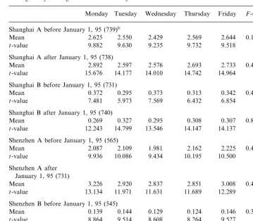
In order to test the trading behavior hypothesis, we compare the trading patterns of stocks with relatively high institutional holdings (B-shares) with those with low institutional holdings (A-shares), while controlling for differences in capitalization. Evidence supporting the dominance of institutional investors in B-share markets is that A-share markets are more volatile than B-shares. A-share prices have a daily standard deviation of around 3.25%, compared with about 2% for B-shares in both exchanges. If there is a relation between the trading pattern and the day-of-the-week effect, it implies that Tuesday’s volume would be less than the volume on the other weekdays. Table 4 presents evidence that does not support this hypothesis. Equality of volume cannot be rejected for all four stock markets in China. Table 4 contains results for turnover by day of the week for these four stock markets in China. The average turnovers are 2.6, 0.32, 2.5 and 0.25% in Shanghai A, Shanghai B, Shenzhen A and Shenzhen B, respectively. The null hypothesis that the mean turnover is the same across all days of the week cannot be rejected.
Eq. (4) is estimated to test explicitly the day-of-the-week effect still exists after
controlling for the monthly effect tested by Wang et al. (1997). An insignificant b1
coefficient will indicate that the return for the first half of the month is not significantly different from that for the last half of the month. A significant negative
b2 coefficient will indicate that the Tuesday return is significantly lower than that
9He discovers that all of the average negative returns from Friday close to Monday close documented
Table 3
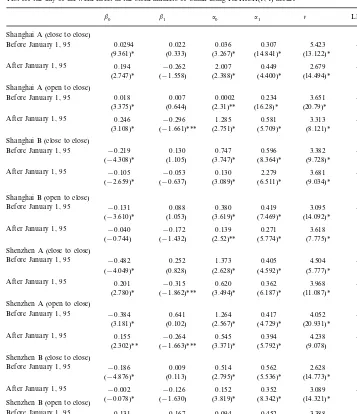
Test for the day-of-the-week effect in the stock markets of China using IGARCH(1, 1) modela
a0 a1 n LR
b1
b0
Shanghai A (close to close)
0.036 0.307 5.423 −2249
Before January 1, 95 0.0294 0.022
(13.122)* (14.841)*
(9.361)* (0.333) (3.267)*
After January 1, 95 0.194 −0.262 2.007 0.449 2.679 −1616
(14.494)* (4.400)*
(2.747)* (−1.558) (2.388)* Shanghai A (open to close)
0.234
0.018 0.007 0.0002 3.651 −2091
Before January 1, 95
(20.79)* (16.28)*
(3.375)* (0.644) (2.31)**
After January 1, 95 0.246 −0.296 1.285 0.581 3.313 −1024
(8.121)* (5.709)*
(2.751)* (3.108)* (−1.661)***
Shanghai B (close to close)
0.747 0.596 3.382 −1404
Before January 1, 95 −0.219 0.130
(−4.308)* (1.105) (3.747)* (8.364)* (9.728)*
After January 1, 95 −0.105 −0.053 0.130 2.279 3.681 −1259
(9.034)* (−2.659)* (−0.637) (3.089)* (6.511)*
Shanghai B (open to close)
Before January 1, 95 −0.131 0.088 0.380 0.419 3.095 −1690
(−3.610)* (1.053) (3.619)* (7.469)* (14.092)*
After January 1, 95 −0.040 −0.172 0.139 0.271 3.618 −912
(2.52)** (5.774)* (7.775)* (−0.744) (−1.432)
Shenzhen A (close to close)
Before January 1, 95 −0.482 0.252 1.373 0.405 4.504 −1446
(−4.049)* (0.828) (2.628)* (4.592)* (5.777)*
After January 1, 95 0.201 −0.315 0.620 0.362 3.968 −1628
(11.087)* (6.187)*
(3.494)* (2.780)* (−1.862)***
Shenzhen A (open to close)
Before January 1, 95 −0.384 0.641 1.264 0.417 4.052 −1142
(20.931)* (4.729)*
(3.181)* (0.102) (2.567)*
After January 1, 95 0.155 −0.264 0.545 0.394 4.238 −1570
(3.371)* (5.792)* (9.078) (2.302)** (−1.663)***
Shenzhen B (close to close)
Before January 1, 95 −0.186 0.009 0.514 0.562 2.628 −813
(14.773)* (5.536)*
(−4.876)* (0.113) (2.795)*
After January 1, 95 −0.002 −0.126 0.152 0.352 3.089 −1224
(14.321)* (−0.078)* (−1.630) (3.819)* (8.342)*
Shenzhen B (open to close)
Before January 1, 95 −0.131 0.167 0.094 0.452 3.388 −499
(13.789)*
(−6.975)* (0.665) (2.23)** (4.376)*
After January 1, 95 −0.004 −0.132 0.146 0.348 3.121 −1217
(8.335)*
(−2.914)* (−1.627) (3.761)* (14.051)*
aTo test whether the day-of-the-week regularity still exist after controlling non-normality of error distribution, the following
IGARCH(1, 1) model is estimated:
rt=b0+b1Tut+ot
o(ot−1,ot−2, …)t
ht=a0+a1ot2−1+a2ht−1, a1+a2=1
where Tu is the dummy variable equal to 1 if datetis Tuesday.t-statistics are in the parentheses. * Denote significant at 1%.
Table 4
Average daily trading volume measured by turnover in the Stock markets of Chinaa
Tuesday Wednesday Thursday Friday F-statistic Monday
Shanghai A before January 1, 95 (739)b
2.429
Mean 2.625 2.550 2.569 2.644 0.102
9.235 9.732 9.518 9.630
9.882
t-value
Shanghai A after January 1, 95 (738)
2.892 2.597 2.576 2.693 2.733 0.472 Mean
t-value 15.676 14.177 14.010 14.742 14.964 Shanghai B before January 1, 95 (731)
0.373
Mean 0.372 0.295 0.313 0.342 0.493
5.973
7.481 7.569 6.432 6.854
t-value
Shanghai B after January 1, 95 (740)
0.269 0.327 0.295 0.308 0.307 0.820 Mean
13.546 14.147 14.137 14.799
t-value 12.243
Shenzhen A before January 1, 95 (565) 2.109
2.087 1.981 2.162 2.225 0.426
Mean
Shenzhen B before January 1, 95 (545)
0.139 0.144 0.129 0.124 0.146 0.388 Mean
9.514
8.864 8.608 8.264 9.527
t-value
Shenzhen B after January 1, 95 (715)
0.315
Mean 0.328 0.372 0.320 0.301 0.294
t-value 7.585 8.871 7.459 7.876 8.082
aTo test the null hypothesis of equal trading volume for each day of the week, the following dummy
variable regressionis estimated:
nt= %
5
k=1 akDkt+et
where nt is the trading volume at datet, Dkt=seasonal dummy for day k(i.e. the dummy variables
indicate the day of the week), andk=Monday (1)–Friday (5).
bNumbers of observations.
on the other 4 days of the week. A significant negative b3 coefficient will indicate
G
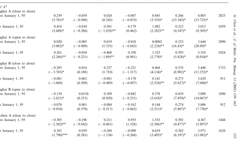
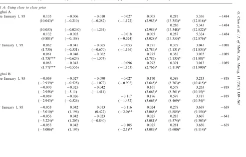
Test for the day-of-the-week effect in the stock markets of China after controlling for other seasonality using IGARCH(1, 1) model
b0 b1 b2 b3 a0 a1 n LR
Panel Ab
Shanghai A (close to close)
0.043
0.259 −0.059 0.024 −0.007 0.266 4.803 2825 Before January 1, 95
(15.345)* (15.725)* (3.519)*
(5.781)* (−0.949) (0.245) (−0.053)
0.416 −0.034 0.501 1.482 0.523 3.015 1059 After January 1, 95 0.179
(4.547)* (9.305)* (3.488)* (−0.206) (−1.828)** (0.462) (2.282)**
Shanghai A (open to close)
0.233 3.644
−0.005 0.019 2090 0.020
Before January 1, 95 −0.018 0.0002
(3.002)* (−0.489) (1.335) (−0.843) (2.224)** (16.43)* (20.89)*
0.593 3.318 1024 After January 1, 95 0.261 −0.034 −0.468 0.350 1.325
(5.828)* (8.034)* (2.778)*
(−0.221) (−1.89)**
(2.266)** (0.981)
Shanghai B (close to close)
−0.221 0.468 0.533 3.448 1753 0.014
Before January 1, 95 −0.205 0.227
(−1.317) (4.134)* (8.902)* (11.252)* (−3.703)* (0.188) (1.710)
0.275 3.629 911
−0.170
−0.081 0.141 After January 1, 95 −0.081 0.062
(5.827)*
(−1.069) (0.589) (−0.489) (−0.697) (2.524)** (7.680)*
Shanghai B (open to close)
0.419 3.098
Before January 1, 95 −0.139 0.0156 0.109 −0.042 0.378 1690 (7.459)* (14.067)*
(3.618)* (−2.621)* (0.215) (0.920) (−0.251)
−0.070 0.061 −0.084 0.144 0.274 3.606 912 After January 1, 95 −0.162
(5.807)*
(−0.910) (0.570) (−0.517) (−0.662) (2.511)* (7.730)*
Shenzhen A (close to close)
0.392 4.367
−0.196 0.211 1444
−0.385
Before January 1, 95 0.955 1.353
(−2.302)** (−0.842) (−0.461) (1.528) (2.566)** (4.477)* (5.897)*
0.181 0.039 −0.268 0.619 0.382 3.971 1626 After January 1, 95 −0.090
(6.197)* (11.082)* (3.495)*
G
Table 5 (Continued)
a1 n LR
b0 b1 b2 b3 a0
Shenzhen A (open to close)
0.406 3.908
−0.202 −0.478 1152 0.165
Before January 1, 95 −0.666 0.207
(−0.307) (1.241) (2.923)** (5.824)* After January 1, 95 0.123 0.064
(5.796)*
(1.321) (0.472) (−0.952) (−0.320) (3.365)* (9.066)*
Shenzhen B (close to close)
0.142 0.509 0.563 2.633 812
−0.175
Before January 1, 95 −0.018 −0.069
(5.557)* (14.703)* (2.801)*
(−3.186)* (−0.243) (−0.581) (0.954)
−0.059 0.106 −0.082 0.147 0.344 3.074 1222 After January 1, 95 −0.087
(−0.565) (−3.799)* (8.315)* (14.563)* (−1.167) (1.523) (−0.772)
Shenzhen B (open to close)
0.422 3.120 547 0.153
Before January 1, 95 0.243 −0.297 −0.492 0.437
(2.077)**
(1.511) (−0.121) (−0.155) (1.077) (7.258)* (15.486)*
0.340 3.106
After January 1, 95 −0.046 0.087 −0.106 −0.055 0.142 1216 (8.277) (14.238)
Shanghai A (close to close)
0.265 4.787 2824 0.046
−0.102 Before January 1, 95 0.252 −0.070 0.032
(3.573)*
(7.244)* (−0.653) (0.425) (−0.468) (15.137)* (15.629)*
0.523 3.026 1059 0.087
−0.419 1.466 After January 1, 95 0.401 0.014
(4.551)*
(4.577)* (0.045) (−2.039)** (0.131) (2.293)** (9.281)*
Shanghai A (open to close)
0.0002
0.018 −0.008 −0.0001 0.051 0.2355 3.652 2089 Before January 1, 95
(16.44)* (20.87)* (2.246)**
(3.488)* (−0.432) (−0.006) (1.311)
0.227 0.156 −0.281 1.286 0.582 3.304 1024 After January 1, 95 −0.147
(−0.242) (2.750)* (5.728)* (8.149)* (2.760)* (0.520) (−1.797)***
Shanghai B (close to close)
0.504 3.453 1751 0.428
Before January 1, 95 −0.185 −0.558 0.109 −0.221
(8.756)*
G
After January 1, 95 0.139
(−0.239) (2.530)** (5.769)* (7.717)* (1.051) (−1.717)***
(−1.261)
Shanghai B (open to close)
0.396 3.092
−0.563 0.085 −0.360 0.348 1686
−0.119 Before January 1, 95
(−3.251)* (−3.306)* (0.995) (−0.986) (3.572)* (7.229)* (14.20)*
−0.106 0.142 0.274 3.605 911 0.236
After January 1, 95 −0.057 −0.163
(5.751)* (7.776)* (2.518)**
(−1.046) (1.004) (−1.802)*** (−0.247)
Shenzhen A (close to close)
0.417 4.452
Before January 1, 95 −0.515 −0.518 0.361 −1.404 1.439 1445 (4.677)* (5.810)*
After January 1, 95 0.197 0.053 −0.308 −0.085
(6.202)*
(2.607)* (0.198) (−1.752)** (−0.132) (3.507)* (11.089)*
Shenzhen A (open to close)
−0.773 0.321 0.426 3.902 1131 Before January 1, 95 −0.311 0.299 −0.320
(6.123)* (11.681)* (0.586)
(−0.161)
(1.141) (−1.171) (−1.641)
0.142 0.158 −0.240 0.551 0.399 4.241 1569 After January 1, 95 −0.259
(−0.424) (3.415)* (5.871)* (9.105)* (2.021)** (0.658) (−1.681)***
Shenzhen B (close to close)
−0.195 0.511 0.561 .628 812
−0.074
Before January 1, 95 −0.182 0.023
(5.524)* (14.719)* (2.782)*
(−4.622)* (−0.505) (0.277) (−0.526)
−0.005 0.021 −0.141 0.153 0.354 3.094 1223 After January 1, 95 0.202
(0.808) (3.831)* (8.381)* (14.258)* (−0.149) (0.177) (−1.718)***
Shenzhen B (open to close)
0.424 3.314
−0.032 0.073 534 0.509
Before January 1, 95 −0.442 0.752
(3.442)* (−0.341) (0.529) (−2.25)* (1.104) (8.709)* (17.710)*
−0.004 0.035 −0.146 0.147 0.352 3.129 1216 After January 1, 95 0.194
(8.371)* (13.964)* (3.772)*
(0.766) (−1.807)***
G
.
Chen
et
al
.
/
J
.
of
Multi
.
Fin
.
Manag
.
11
(2001)
139
–
163
Table 5 (Continued)
at-statistics are in the parentheses.
bTo test explicitly whether the day-of-the-week effect still exists after controlling for the effect of Tuesdays in the last-half of the month, we estimate the
following regression:
rt=b0+b1LHMt+b2Tut+b3LHMt*Tut+ot
o(ot−1,ot−2, …)t
ht=a0+a1ot2−1+a2ht−1, a1+a2=1
where LHM is the last-half month variable that takes a value of 1 if the return is for the last half of the month and Tu is the all Tuesdays variable that takes a value of 1 if the return occurs on a Monday. LHM*Tu is the last-half month Tuesdays variable that takes a value of 1 if the Tuesday falls in the last half of the month.
cTo test explicitly whether the day-of-the-week effect still exists after controlling for the January effect and the Tuesdays in January, we estimate the
following regression:
rt=b0+b1JANt+b2Tut+b3JANt*Tut+ot
o(ot−1,ot−2, …)t
ht=a0+a1ot2−1+a2ht−1, a1+a2=1
where JAN is the January variable that takes a value of 1 if the return is in January and Tu is the all Tuesdays variable that takes a value of 1 if the return occurs on a Tuesday. JAN*Tu is the January Tuesdays variable that takes a value of 1 if the Tuesday falls in January.
stock returns for the first half of the month in China. The coefficients of the Tuesday variable, except for Shanghai A, are not significantly negative after January 1, 1995 for all four stock markets. This results indicates that, after controlling for the monthly effect, the stock returns on Tuesdays are not lower than the returns of the other 4 days.
To test explicitly whether the day-of-the-week effect still exists after controlling for the January effect and the Tuesdays in January, we estimate Eq. (5). An insignificant b1 coefficient will indicate that the return for January is not
signifi-cantly different from the other months. A significant negative b2 coefficient will
indicate that the Tuesday return is significantly lower than that of the other 4 days
of the week. A significant negative b3 coefficient will indicate that return on
Tuesdays during January is not lower than that in other months. Panel B of Table 5 reports the regression results. The coefficients of January variable are generally negative and statistically insignificant before January 1, 1995 for all four markets, while the coefficients of the January variable are generally positive and statistically insignificant for the second sub-period. The results indicate that the stock returns in January are not statistically different from the stock returns in other months in China. The coefficients of Tuesday variable are significantly negative after January 1, 1995 for all four stock markets. This results indicates that, after controlling for the January effect, the stock returns on Tuesdays are still lower than the returns on the other 4 days.
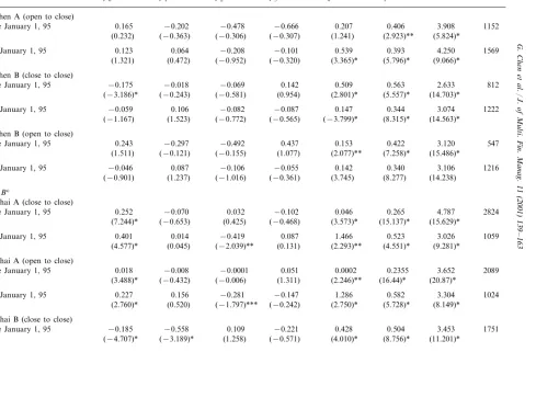
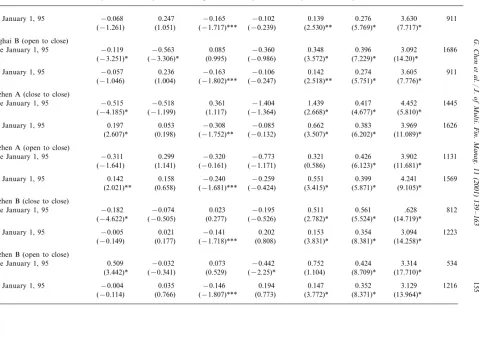
We examine the spillover hypothesis by estimating regression 6. The results are reported in Table 6. We find evidence that returns on Tuesday are generally insignificantly negative for both sub-periods after taking the spillover effect into account. This result in Table 6 provides evidence of a potential link in the day-of-the-week effect and interactions across international markets. We speculate that the disappearance of the day-of-the-week effect after controlling for spillover from U.S. and Hong Kong stocks may be due to the fact that the Chinese economy because relatively more involved with international business and more open to the outside after 1995.
5. Conclusion
G
Test for the day-of-the-week effect in the stock markets of China after considering the spillover impact from U.S. and Hong Kong stock marketsa
b1 b2 b3 b4 a0 a1 n LR
Panel A:Using close to close price
Shanghai A
0.135 −0.006 −0.010 −0.027 0.005 0.287
Before January 1, 95 5.336 −1484 (10.043)* (−0.210) (−0.282) (−1.122) (2.983)* (13.353)* (12.816)*
After January 1, 95 0.271 0.379 3.043 −1088 (1.750) (−0.531) (−0.670) (−1.146) (2.784)* (5.131)* (11.834)*
Before January 1, 95 −818 (−2.939)* (−0.528) (−1.072) (−0.902) (3.645)* (8.363)* (10.415)*
After January 1, 95 0.024 0.278 3.639 −639 (−3.010)* (1.196) (0.427) (−2.0)** (3.068)* (6.885)* (9.154)*
−0.056 0.042 −0.023 0.025 0.283 3.607 −641 (−3.224)* (1.203) (−0.840) (3.081)* (6.574)* (9.303)*
G
Before January 1, 95 0.023 0.040 0.231 0.394 5.051 −980 (−3.743)* (0.730) (0.130) (0.627) (2.665)* (4.628)* (5.245)*
−0.199 0.097 0.043 0.231 0.395 5.050 −980 (−3.755)* (0.746) (0.684) (2.668)* (4.634) (5.246)*
−0.197 0.097 0.056 0.230 0.394 5.042 −980 (−3.801)* (0.738) (0.320) (2.658)* (4.625)* (5.271)*
0.079 −0.137 0.055 0.056
After January 1, 95 0.106 0.386 4.030 −1015 (2.598)* (−1.917)*** (0.678) (1.440) (3.634)* (6.485)* (11.298)*
0.080 −0.133 0.067 0.105 0.383 4.028 −1015 (2.637)* (−1.875)*** (1.99)** (3.618)* (0.6451)* (11.316)*
0.077 −0.137 0.102 0.105 0.385 4.025 −1016 (2.551)* (−1.926)*** (1.431) (3.639)* (6.515)* (11.278)*
Shenzhen B
−0.077 0.003
Before January 1, 95 0.006 0.011 0.069 0.499 2.714 −370 (−4.837) (0.077) (0.118) (0.615) (2.905)* (5.912)* (14.566)*
−0.077 0.003 0.012 0.069 0.497 2.713 −376 (−4.855)* (0.105) (0.688) (2.901)* (5.896)* (14.596)*
−0.078 0.004 0.016 0.070 0.502 2.711 −376 (−4.886)* (0.119) (0.315) (2.909)* (5.930)* (14.582)*
−0.005 −0.031 −0.062
After January 1, 95 0.072 0.026 0.339 2.111 −674 (−0.387) (−0.986) (−1.439) (2.917)* (3.843)* (8.447)* (21.148)*
−0.006 −0.037 0.056 0.026 0.335 3.079 −642 (−0.461) (−1.189) (2.521)* (3.827)* (8.470)* (15.064)*
−0.004 −0.034 −0.002 0.023 0.324 3.096 −645 (−0.324) (−1.086) (−0.041) (3.795)* (8.434)* (14.973)*
Panel B:Using open to close price
Shanghai A
−0.021
Before January 1, 95 0.0003 0.003 −0.004 0.0004 0.276 3.495 −1478 (−4.053)* (0.034) (0.599) (−0.738) (2.772)* (14.88)* (19.94)*
−0.018 −0.005 −0.004 0.0004 0.277 3.484 −1479 (−3.393)* (−0.502) (−1.123) (2.281)* (14.852)* (20.084)*
G
After January 1, 95 0.009 0.966 0.422 3.271 −1501 (−1.511) (1.419) (−0.730) (0.123) (2.738)* (5.039)* (9.622)*
Before January 1, 95 0.471 0.406 2.957 −1280 (3.173)* (−1.033) (−3.920)* (−0.609) (3.044)* (6.033)* (13.390)*
After January 1, 95 −0.064 0.109 0.244 3.639 −1200 (3.240)* (0.373) (−6.076)* (−1.194) (2.898)* (5.935)* (8.604)*
0.129 0.019 −0.192 0.108 0.246 3.685 −1200 (3.162)* (0.227) (−7.773)* (2.901)* (5.918)* (8.386)*
0.114 0.087 −0.185 0.119 0.261 3.685 −1215 (2.795)* (1.015) (−3.88)* (2.996)* (96.305)* (8.654)*
Shenzhen A
0.115 −0.161
Before January 1, 95 0.174 0.417 0.001 0.850 2.346 −1351 (0.456) (−0.324) (0.785) (0.963) (0.002) (10.34)* (13.54)*
0.239 −0.109 0.108 0.002 0.853 2.343 −1348 (0.564) (0.432) (0.587) (0.001) (10.86)* (14.32)*
0.202 −0.071 0.725 0.001 0.890 2.330 −1349 (0.365) (−0.123) (0.879) (0.001) (11.19)* (13.68)*
0.155 −0.262 0.054
After January 1, 95 0.016 0.562 0.402 4.218 −1535 (2.267)** (−1.621) (1.426) (0.207) (3.326)* (5.682)* (9.092)*
0.156 −0.258 0.057 0.562 0.402 4.216 −1535 (2.282)** (−1.615) (1.71)*** (3.323)* (5.679)* (9.090)*
G
.
Chen
et
al
.
/
J
.
of
Multi
.
Fin
.
Manag
.
11
(2001)
139
–
163
161
b1 b2 b3 b4 a0 a1 n LR
Shenzhen B
−0.287 −0.569
Before January 1, 95 −0.179 −0.103 0.001 0.843 2.292 −1472 (−0.781) (−0.852) (−0.369) (−0.147) (0.001) (9.64)* (14.32)*
0.125 0.138 −0.321 0.002 0.847 2.329 −1475 (−0.528) (0.471) (0.845) (0.003) (9.67)* (13.96)*
−0.284 0.107 −0.102 0.001 0.837 2.292 −1773 (0.785) (0.356) (−0.167) (0.001) (9.87)* (13.96)*
−0.004 −0.116 0.088
After January 1, 95 −0.073 0.162 0.352 3.084 −1211 (−0.123) (−1.502) (3.498)* (−1.672) (3.759)* (8.132)* (14.484)*
−0.006 −0.014 0.069 0.161 0.353 3.075 −1212 (−0.166) (−1.819)*** (3.069)* (3.738)* (8.153)* (14.494)*
−0.0005 −0.133 0.003 0.146 0.348 3.121 −1217 (−0.015) (−1.735)*** (0.088) (3.760)* (8.321)* (14.054)*
aIn order to test the spillover hypothesis, the following IGARCH(1, 1) model is estimated:
rt=b1+b2Tut+b3HKt+b4USt−1+ot
o(ot−1,ot−2, …)t
ht=a0+a1ot2−1+a2ht−1, a1+a2=1
where Tu is the dummy variable equal to 1 if datetis Tuesday, HKtis return on the Heng Seng Index at datetand USt−1is return on the Dow Jones
Industrial Index at datet−1.t-statistics are in the parentheses. * Denote significant at 1%.
the Pacific by 1 day but not in the opposite direction. This result suggests that information flows primarily from the Americas to Europe and Asia. If this result holds, we would expect the U.S. stock market to lead China’s stock markets. Wang et al. (1997), Chang et al. (1998) find the day-of-the-week effect exists in the U.S. markets after 1990s. This Tuesday anomaly disappears after taking the non-normal-ity distribution and spillover from other countries into account. Our finding suggests that this day-of-the-week regularity in China may be due to the spillover from the Americas. The evidence of the day-of-the-week anomaly in China is clearly dependent on the estimation method and sample period. When transaction costs are taken into account, the probability that arbitrage profits are available from the day-of-the-week trading strategies seems very small. This conclusion is obviously consistent with an efficient market approach. Hopefully our study provides some insight and understanding of stock markets in China and the day-of-the-week regularity.
Acknowledgements
This study was substantially supported by a grant from the Departmental Research Grant of Hong Kong Polytechnic University (Account No. A-PA 15). Chuck Kwok also gratefully acknowledges the support of the Center for International Business Education and Research (CIBER) at the University of South Carolina.
References
Abraham, A., Ikenberry, D.L., 1994. The individual investor and the weekend effect. Journal of Financial and Quantitative Analysis 29, 263 – 277.
Aggarwal, R., Rivoli, P., 1989. Seasonal and day-of-the-week effects in four emerging stock markets. Financial Review 24, 541 – 550.
Ariel, R., 1987. A monthly effect in stock returns. Journal of Financial Economics 18, 161 – 174. Baillie, R.T., Bollerslev, T., 1989. The message in daily exchange rates: a conditional variance tale.
Journal of Business and Economic Statistics 7, 297 – 305.
Barone, E., 1990. The Italian stock market efficiency and calendar anomalies. Journal of Banking and Finance 14, 483 – 510.
Bollerslev, T., 1987. A conditionally heteroskedastic time series model for speculative prices and rates of return. Review of Economics and Statistics 69, 542 – 547.
Chang, E.C., Pinegar, J.M., Ravichandran, R., 1998. US day-of-the-week effects and asymmetric responses to macroeconomic news. Journal of Banking and Finance 22, 513 – 534.
Chui, A., Kwok, C., 1998. Cross-autocorrelation between A shares and B shares in the Chinese stock market. Journal of Financial Research 21, 333 – 353.
Connolly, R., 1989. An examination of the robustness of the weekend effect. Journal of Financial and Quantitative Analysis 24, 133 – 169.
Copeland, M., Copeland, T., 1998. Leads, lags, and trading in global markets. Financial Analysts Journal, 1998, July/August, 55, 70 – 80.
Dubois, M., Louvet, R., 1996. The day-of-the-week effect: the international evidence. Journal of Banking and Finance 20, 1463 – 1484.
Dyl, E.A., Marberly, E.D., 1988. A possible explanation of the weekend effect. Financial Analyst Journal, May – June, 44, 83 – 84.
Engle, R.F., Bollerslev, T., 1986. Modelling the persistence of conditional variances. Econometric Review 5, 1 – 50.
French, K., 1980. Stock returns and the weekend effect. Journal of Financial Economics 8, 55 – 69. French, K.R., Schwert, G.W., Stambaugh, R.R., 1987. Expected stock returns and volatility. Journal of
Financial Economics 19, 3 – 29.
Gibbons, M., Hess, R., 1981. Day of the week effects and asset returns. Journal of Business 54, 579 – 596. Harris, L., 1986. A transaction data study of weekly and intradaily patterns in stock returns. Journal of
Financial Economics 16, 99 – 117.
Jaffe, J., Westerfield, R., 1985a. The weekend effect in common stock returns: the international evidence. Journal of Finance 40, 433 – 454.
Jaffe, J., Westerfield, R., 1985b. Patterns in Japanese common stock returns: day of the week and turn of the year effects. Journal of Financial and Quantitative Analysis 20, 243 – 260.
Keim, D., 1983. Size-related anomalies and stock return seasonality: further empirical evidence. Journal of Financial Economics 12, 13 – 32.
Keim, D.B., Stambaugh, R.F., 1984. A further investigation of the weekend effect in stock returns. Journal of Finance 39, 819 – 835.
Lakonishok, J., Levi, M., 1982. Weekend effects in stock returns: a note. Journal of Finance 37, 883 – 889.
Lakonishok, J., Marberly, E., 1990. The weekend effect: trading patterns of individual and institutional investors. Journal of Finance 45, 231 – 243.
Lakonishok, J., Smidt, S., 1984. Volume and turn-of-the-year behavior. Journal of Financial Economics 13, 435 – 455.
McCurdy, T., Morgan, I., 1987. Tests of the Martingale hypothesis for foreign currency features with time-varying volatility. International Journal of Forecasting 3, 131 – 148.
Patell, J., Wolfson, M., 1982. Good news, bad news, and the intraday timing of corporate disclosures. Accounting Review 57, 509 – 527.
Rogalski, R., 1984. A further investigation of the weekend effect in stock returns. Journal of Finance 39, 835 – 837.
Smirlock, M., Starks, L., 1986. Day-of-the-week and intraday effects in stock returns. Journal of Financial Economics 17, 197 – 210.
Sias, R.W., Starks, L.T., 1995. The day-of-the-week anomaly: the role of institutional investors. Financial Analysts Journal, May – June, 51, 58 – 67.
Theobald, M., Price, V., 1984. Seasonality estimation in thin markets. Journal of Finance 39, 377 – 392. Wang, K., Li, Y., Erickson, J., 1997. A new look at the Monday effect. Journal of Finance 52,
2171 – 2186.