E l e c t ro n ic
Jo u r n
a l o
f P
r o b
a b i l i t y
Vol. 6 (2001) Paper no. 18, pages 1–19. Journal URL
http://www.math.washington.edu/˜ejpecp/ Paper URL
http://www.math.washington.edu/˜ejpecp/EjpVol6/paper18.abs.html
INVARIANT WEDGES FOR A TWO-POINT REFLECTING BROWNIAN MOTION AND THE “HOT SPOTS” PROBLEM
Rami Atar
Department of Electrical Engineering, Technion – Israel Institute of Technology Haifa 32000, Israel
[email protected] AbstractWe consider domainsDofR
d,d≥2 with the property that there is a wedgeV ⊂ R
d
which is left invariant under all tangential projections at smooth portions of ∂D. It is shown that the difference between two solutions of the Skorokhod equation inDwith normal reflection, driven by the same Brownian motion, remains in V if it is initially inV. The heat equation on Dwith Neumann boundary conditions is considered next. It is shown that the cone of elements uof L2(D) satisfyingu(x)−u(y)≥0 wheneverx−y∈V is left invariant by the corresponding heat semigroup. Positivity considerations identify an eigenfunction corresponding to the second Neumann eigenvalue as an element of this cone. For d = 2 and under further assumptions, especially convexity of the domain, this eigenvalue is simple.
Keywords Reflecting Brownian motion, Neumann eigenvalue problem, Convex domains. AMS subject classification 35K05 (35B40, 35B50, 35J25, 60H10)
1
Introduction
The “hot spots” property of a bounded connected open domainD⊂R
d refers to the location of the extrema of eigenfunctions corresponding to the second eigenvalue of the Laplacian onDwith Neumann boundary conditions. Among the various statements associated with this property [1, 3, 5, 10, 11] let us mention:
(HS) Every eigenfunction corresponding to the second Neumann eigenvalue attains its extrema solely on the boundary.
(HS’) There exists an eigenfunction corresponding to the second Neumann eigenvalue which attains its extrema solely on the boundary.
The name comes from considering the heat equation on D:
Under weak assumptions onDan eigenfunction expansion for the solutions of the heat equation is available. Since the eigenfunction corresponding to the first eigenvalue is a constant, the spatial locations of extrema of the solution for a typical initial condition are governed at large values of tby the second eigenspace. The assertion is therefore on the “hottest” and “coldest” spots inD.
Although it has been shown that (HS) holds for special domains by direct calculation, there are large classes of domains about which little is known. For example, for a planar simply connected domain with smooth boundary and no line of symmetry, there is no known criterion (to the author’s best knowledge) to check whether (HS) is satisfied, other than calculation when it is possible. In [5] an example was first found of a domain that does not satisfy (HS), and in [3] an example was found of a domain for which the second Neumann eigenvalue (which we denote by µ2 in what follows), is simple, and the corresponding eigenfunction attains both its strict extrema in the interior. See [1] for a conjecture that (HS) holds for all convex planar domains, and [5] for a conjecture that it holds for planar domains with at most one hole.
In dimension greater than two, the only domains known to satisfy the hot spots property, other than domains with special symmetry, are those of the formD′×[0, a] (see Kawohl [11]), or more generally D′ ×D′′ (see [1]). One of our two goals is provide new classes of domains in higher
dimension satisfying (HS’). What might naively be expected to be the extension of the result of [1] regarding the coupled Brownian motions, does not hold. For example, the condition that all unit normals to ∂D at its smooth portions form scalar product with a fixed vector within the range of (−ǫ, ǫ), does not guarantee that there is an invariant set for the coupled processes, in the sense described above, no matter how smallǫ > 0 is. We show that the approach of [1] can be generalized in a different way. Our assumption onDis that it is piecewise smooth with “convex corners” (see Condition 2.1). We then assume there is a wedgeV ⊂R
d (see Definition 2.1) that is left invariant under all projections onto subspaces tangential to∂D at smooth portions. We prove that two reflecting Brownian motions coupled as described above have difference in V if initialized there. As a result, the Neumann heat semigroup leaves the following cone of L2(D) invariant:
{u∈L2(D) :u(x)−u(y)≥0, x, y∈D, x−y∈V}. (2) Invoking positivity considerations the following is shown (see Theorem 3.1).
Assume that for some γ ∈R
d one has hv, γi>0 for all v∈V. Then there is an eigenfunction
corresponding to the second Neumann eigenvalue attaining both strict extrema on the boundary.
(HS) follows from (HS’) whenever it is known that µ2 is simple. In a sense, it is typical that µ2 is simple, as can be seen e.g. in [15]. It is known also that for simply connected planar domains, the multiplicity is at most two [16]. However, for a given domain it is in general hard to determine whether an eigenvalue is simple. An exception is a result that appears in [1], where it is shown that µ2 is simple for convex planar domains for which the diameter to width ratio exceeds a certain number.
In this paper we identify a new class of planar domains for whichµ2 is simple. It is a subclass of the planar domains for which we prove that (HS’) holds (with V =R
2
+). As a result, they satisfy (HS). We show (see Theorem 4.1)
Let Dbe a planar open domain bounded between the graphs of two C2 increasing functions, one of which is convex and the other concave, such that Dis bounded. Assume that for each corner point Ξ of the domain, Br(Ξ)∩D is a sector for some r >0, of angle within [π/4, π/2). Then
the second Neumann eigenvalue on D is simple.
2
An invariance property
In this section we use the results of Lions and Sznitman [14] that guarantee the existence of a unique solution to the Skorokhod problem for arbitrary continuous paths. We prove a certain invariance property in continuous paths space, which then translates to a property of semimartingale reflecting Brownian motions.
We will always consider domains that satisfy the following. Condition 2.1 D⊂R
d is a bounded, connected domain with Lipschitz boundary, and is given
by the intersection of a finite collection {Di}i∈I of open sets with C2 boundary.
For domains satisfying Condition 2.1 we will consider the vector fieldnof unit inward normals. The (not necessarily single-valued) vector fieldnis defined on the boundary∂DofDas follows. For x ∈ ∂Di let nx,i denote the unit inward normal to ∂Di at x. Then for x ∈ ∂D we let Ix={i∈I :x∈∂Di} and
n(x) ={ν:ν =X i∈Ix
ainx,i, |ν|= 1, ai ≥0, i∈Ix}.
We remark that the definition of [14] (equation (1) p. 514) of a vector field for a more general class of domains reduces to the above definition for the domains considered here.
The setN =N(D) is defined as
N ={nx,i:i∈Ix, x∈∂D}. (3)
Forn∈N, then-projectionπn:R d →
R
d is defined as πnv=v− hv, nin. For x, y ∈ R
d, let xy denote the closed line segment xy = {αx+ (1−α)y : α ∈ [0,1]}. Let W =W(D) be defined by
W ={x−y:x, y∈D, xy¯ 6⊂D¯}.
Definition 2.1 A proper subsetV of R
d is called awedgeif it is closed, convex, has non-empty
interior, and if v∈V implies αv ∈V for allα≥0.
The most significant assumption we make is the following.
Condition 2.2 There exists a wedge V satisfying W ⊂V ∪ −V, and
v∈V, n∈N =⇒πnv∈V.
We will say that a wedge V is invariant for D if it satisfies Condition 2.2. We next formulate an equivalent to Condition 2.2.
Condition 2.2′ There exists a wedge V satisfying W ⊂V ∪ −V, and
v∈∂V, n∈N =⇒ hm, nihn, vi ≤0,
Proposition 2.1 Conditions 2.2 and 2.2′ are equivalent. with non-empty interior, every neighborhood ofv contains a point in the interior. Since Vc is open andπn continuous, there is a pointw∈Vo for which u=. πnw∈Vc. The convexity of V implies that the line segmentwu intersects∂V at exactly one point, sayz. There must exist an inward normal ˜m to ∂V at z such that hm, w˜ −zi>0, and consequentlyhm, u˜ −zi<0. Note however that πnw =πnz= u. Hence hm, π˜ nz−zi <0 and it follows that hm, n˜ ihn, zi > 0, in contradiction with Condition 2.2′. Therefore Condition 2.2 holds.
The definition of a solution to the Skorokhod problem for an arbitrary continuous function follows [14]. The notation |h|t is for the total variation of a function h : [0,∞) → R
d on [0, t] with respect to the Euclidean norm on R
d.
Definition 2.2 For w ∈ C([0,∞) : R
d) such that w(0) ∈ D¯ we say that the pair (x, l) solves the Skorokhod problem (w, D, n) if the conditions listed below are satisfied.
x∈C([0,∞),D¯), l∈C([0,∞),R
The following result is a special case of [14] Theorem 2.2 (see also [14] Remark 2.4 regarding domains with convex corners; the uniform exterior sphere condition obviously holds).
Theorem 2.1 (Lions and Sznitman) Let D ⊂ R
and note that it is of bounded variation on any bounded interval.
Note that every wedge may occupy no more than a half space i.e., there must exist aγ ∈R d for which hv, γi ≥0 for all v∈V. The following condition is slightly stronger.
Condition 2.3 There exists a γ ∈R
d such that for every v∈V \ {0}, hv, γi >0.
Theorem 2.2 Assume Conditions 2.1 and 2.2 hold, let V be an invariant wedge for D and assume that it satisfies Condition 2.3. Then if δ0 ∈V, one has δt∈V for all t >0.
Let V be some set satisfying Condition 2.2. We define on Vc a vector field m as follows. For each ǫ >0 letVǫ be the open convex subset of R
d defined by Vǫ={v ∈R
d : dist(v, V)< ǫ}. (5)
For each v∈Vc let m(v) be the unit inward normal to∂Vǫ at v, withǫ= dist(v, V). Note that the function is well defined since the normal is unique.
Lemma 2.1 Let u: [s, t]→Vc be continuous and of bounded variation. Then
dist(u(t), V)−dist(u(s), V) =
Z t
s h−
m(u(θ)), du(θ)i. (6)
Proof: We first show that the integral on the right is well defined by showing that m(u(θ)) is in fact continuous in θ. It is enough to show that m(u) is continuous in u. The proof of this fact is elementary and for completeness we have included it in the appendix (see Lemma 5.1). Defineψ:Vc →
R
d byψ(x) = dist(x, V). It is elementary to show that for anyr∈ R
d,|r|= 1, andx∈Vc, the directional derivative ofψatxsatisfies limǫ↓0ǫ−1(ψ(x+ǫr)−ψ(x)) =h−m(x), ri. This shows that ∇ψ(x) is well defined and is equal to −m(x). Sincem is continuous ψ is C1, and it follows that
ψ(u(t))−ψ(u(s)) =
Z t
s h∇
ψ(u(θ)), du(θ)i
which proves the lemma.
Below, we borrow some ideas from the proof of [8] Theorem 2.2.
Proof of Theorem 2.2: Letu∈∂Vǫ and m=m(u). We first show that for all n∈N
hm, nihn, ui ≤ −ǫhm, ni2. (7)
Letv=u+ǫm. Then it is easy to see that v∈∂V and that mis an inward normal to ∂V at v. By Proposition 2.1, Condition 2.2′ holds. Hence hm, nihn, vi ≤ 0, n∈N and the estimate (7) follows.
Assume that the conclusion of the theorem does not hold. Note that δs = 0 implies δt = 0, t > s. Note also that by Condition 2.3 there is a γ such that for v ∈ V either hv, γi > 0 or v= 0. Hence there must exists, tsuch that for all θ∈[s, t], δθ∈Vc∩ {u:hu, γi>0}and such that dist(δt, V)>dist(δs, V). It follows from Lemma 2.1 that
Z t
s h
m(δθ), νθxid|lx|θ <
Z t
s h
whereνθx ∈n(xθ), νθy ∈n(yθ), θ∈[s, t]. Therefore there must exist a θ∈[s, t] such that either (a) hm(δθ), νθxi<0 and xθ ∈∂D;
or
(b) hm(δθ), νθyi>0 and yθ∈∂D. Since the argument is similar in both cases, we only consider case (a).
On one hand, one has in case (a) thathm(δθ), νi <0 for ν=nxθ,i and somei∈Ixθ. Hence by (7), hν, δθi>0. On the other hand, sinceW ⊂V ∪ −V and hδθ, γi>0 one has that δθ 6∈W. It follows thatxθyθ⊂D¯. Thereforehδθ, νi ≤0 for every ν∈n(xθ). This is a contradiction. We close this section by showing an implication to reflecting Brownian motion. On a complete probability space (Ω, F, P) with an increasing family of sub σ-fields (Ft)t≥0 let (Wt)t≥0 be a d-dimensional Ft-Brownian motion.
The following result is proved in [14] (condition [14](9) holds by Remark [14] 3.9).
Theorem 2.3 (Lions and Sznitman) Let D satisfy Condition 2.1 and let x0 ∈D¯ be given.
Then there exists a unique continuousFt-semimartingale (Xt)t≥0 = (Xtx0)t≥0 satisfying:
There exists an R
d-valued continuous bounded variation process L t
such that for all t≥0 a.s. Xt∈D,¯
Xt=x0+Wt+Lt, (8)
|L|t=
Z t
0
1Xs∈∂Dd|L|s,
Lt=
Z t
0
ξsd|L|s with ξs∈n(Xs).
The conclusion of Theorem 2.3 is equivalent to the statement that for a.e. ω∈Ω, (X, L) solves the Skorokhod problem (x0+W, D, n) (see e.g., Remark 3.2 of [14]).
Letx0, y0 ∈D¯. A two-point semimartingale reflecting Brownian motion in ¯Dstarted at (x0, y0) is a pair (Xt, Yt) ofFt-semimartingales as in Theorem 2.3 with (Xt) = (Xtx0) and (Yt) = (Xty0). Note that by definition X and Y are driven by the same process W, but have different initial conditions, x0 andy0.
From Theorems 2.2 and 2.3 we obtain the following.
Corollary 2.1 Let (Xt, Yt) be a two-point semimartingale reflecting Brownian motion in D¯
started at (x0, y0)∈D¯ ×D¯. Let the assumptions of Theorem 2.2 hold. Ifx0−y0 ∈V then a.s., Xt−Yt∈V for allt >0.
In what follows we will denote by Px,y the probability measure on (Ω, F,(Ft)) for which Px,y[(X0, Y0) = (x, y)] = 1. Px will denote the restriction of Px,y to the σ-field generated by X·. Ex,y and respectively,Ex will denote expectation with respect toPx,y and Px.
3
Positivity considerations for the heat semigroup
Consider the heat equation with Neumann boundary conditions (1), the corresponding heat kernelpt(x, y), and the semigroupTtthat it generates. Under Condition 2.1,p1(x, y) is uniformly bounded, Tt maps L2(D) into L∞(D) and has a discrete spectrum on L2(D) (see e.g., [1]). Let φ11, . . . , φk1
1 , φ12, . . . , φk
2
2 , . . . denote an orthonormal basis for L2(D) of eigenfunctions with eigenvalues µ1 < µ2 < µ3 < . . ., where µi corresponds to φji. Recall that k1 = 1, µ1 = 0 and φ11= 1/vol(D). In this section we prove the following result.
Theorem 3.1 Assume Conditions 2.1 and 2.2 hold, let V be an invariant wedge for D and assume that it satisfies Condition 2.3. Then there is an eigenfunction φ2 corresponding to the
second Neumann eigenvalue µ2, satisfying φ2(x) ≥ φ2(y) whenever x, y ∈ D and x−y ∈ V.
Moreover, for ally ∈D
inf
x∈∂Dφ2(x)< φ2(y)<xsup∈∂Dφ2(x). (9) What provides the link between the heat equation and the reflecting Brownian motion is that ifu solves (1) then
u(t, x) =Exu0(Xt) (10)
holds true whenever u0 ∈ C(D)∩L2(D). The proof of this fact follows that of [2] Theorem 4.14 where Dirichlet boundary conditions are considered. The estimate needed there on the eigenvalues easily follows from e.g. [1] p. 8. Finally, the boundary conditions are satisfied since by [4] Lemma 4.3(a) the transition density satisfies them.
Let nowU denote the orthogonal complement to the first eigenspace inL2(D) i.e.,
U ={u∈L2(D) :
Z
D
u(x)dx= 0}.
Let the restriction ofTt to U be denoted by ˆTt. Define
S ={u∈U :u(x)≥u(y), x, y ∈D, x−y∈V}.
The following argument was introduced in [1] (in a slightly different context). As a result of Corollary 2.1 and equation (10), we have that u(t, x)−u(t, y) =Ex,y(u0(Xt)−u0(Yt)) hence
ˆ
Ttu0 ∈S whenever u0 ∈S is continuous. Since S is closed in U and ˆTt continuous we have, in fact, that ˆTtS ⊂S. Note also that the spectral radius of ˆTtis e−µ2t.
We recall an abstract result on linear operators that leave a cone invariant. Let E be a real normed space. A closed setK⊂Eis called aconeif for alla, b∈K,α≥0 one hasa+b, αa∈K, and if K∩ −K contains only the zero vector. Ifa, b∈E andb−a∈K, one writesa≤b. The following is from [12] Theorem 9.2.
Theorem 3.2 Let A be an operator in a real Banach space E that leaves a cone K invariant (i.e., AK ⊂K). Assume
i. K−K=E,
Then r(A) is an eigenvalue of A with a corresponding eigenvector inK.
Proof of Theorem 3.1: We verify the hypotheses of Theorem 3.2. The fact thatS∩−S={0} follows easily from the assumption thatV has a nonempty interior. HenceS is obviously a cone in the Banach space U with the norm ofL2(D). To show that S−S =U it is enough to show that every u ∈ U that satisfies a global Lipschitz condition can be written as the difference between two elements ofS. Assume then that
|u(x)−u(y)| ≤κ|x−y|, x, y∈D.
By Condition 2.3 there must beγ andǫ >0 such thathv, γi ≥ǫ|v|for allv∈V. Letx0 be such thatR
Dhx−x0, γidx= 0 and let z(x) =hx−x0, γi. Then
u(x)−u(y) +κǫ−1hγ, x−yi ≥0 (11) for all x, y ∈D, x−y ∈ V. That is, u+κǫ−1z ∈ S. Obviously z ∈ S, hence we obtain that S−S =U. As discussed before, ˆTt leaves S invariant. Moreover, r( ˆTt) =e−µ2t>0. Hence by Theorem 3.2 there is an eigenfunction φ2 inS, corresponding toµ2.
To conclude (9) we proceed as in the proof of Theorem 3.3 of [1]. Every eigenfunction must be real analytic in D [1] hence cannot be constant in an open set unless it is identically zero. However, ifyis any interior point then φ2(y)≤φ2(x) ifx belongs to the set (y+V)∩D, which has non-empty interior. Consequently, φ2 cannot attain its maximum at y.
4
Simplicity in dimension two
In this section we deal solely with planar domains. It is known since [16] that the multiplicity of µ2 for simply connected planar domains is at most two. For a certain family of planar domains we prove that µ2 is simple.
Theorem 4.1 Let D be a bounded domain of the form
D={x∈R 2 :g(x
1)< x2 < h(x1)},
where g and h are non-decreasing C2 functions, g is convex and h concave. Let (ξ1, g(ξ1))
and (ξ2, g(ξ2)) denote the two corner points (i.e., ξ1 and ξ2 are the only two solutions ξ to the
equation g(ξ) =h(ξ)). Assume that for i= 1,2, both g and h are affine at some neighborhood of ξi and the angle between the graphs of g and h near ξi is greater than or equal toπ/4. Then
the second Neumann eigenvalue on D is simple.
Before proving the above result, let us show that Theorem 3.1 can be applied to domains inR 2 to recover the following result of [1], section 3, specialized to domains with convex corners. Theorem 4.2 (Ba˜nuelos and Burdzy) Let g, h : [0, a]→R be nondecreasing and such that
bothgand−h are given by the maximum over a finite collection of continuous functions on[0, a]
that areC2 on(0, a). Assume thatg < hon(0, a) whileg=hon {0, a}, and thatg(0+)< h(0+), g(a−)< h(a−). Let
D={x∈R 2 :g(x
Then there is an eigenfunction corresponding to the second Neumann eigenvalue onDsuch that for ally ∈D
inf
x∈∂Dφ2(x)< φ2(y)<xsup∈∂Dφ2(x).
Proof: We will show that the assumptions of Theorem 3.1 are satisfied. Condition 2.1 trivially holds. Let V = R
2
+. Then it is obvious that V is a wedge and that W ⊂ V ∪ −V. By monotonicity, the inward normal at smooth portions of the boundary always satisfies
hn, e1ihn, e2i ≤0.
Note that whenever v ∈ ∂V \ {0} and m is an inward normal to ∂V at v then either v is a positive multiple of e1 and m =e2 orv is a positive multiple of e2 and m =e1. Hence in view of the last display, Condition 2.2′ holds, andV is an invariant wedge forD. Condition 2.3 holds trivially. The conclusions of Theorem 3.1 are therefore valid.
Remark: Let mg = supg′ and mh = suph′ where the supremum is over all smooth points. Then it is easy to see that the set{x : 0≤x2 ≤max(mg, mh)x1}is an invariant wedge forDas well.
We introduce some notation. Consider the Banach space ˜U of functions on D that satisfy a global Lipschitz condition as well as
Z
D
u(x)dx= 0,
equipped with the norm
kuk∼= sup x∈D|
u(x)|+ sup x,y∈D:x6=y
|u(x)−u(y)|
|x−y| .
Similarly to the definition ofS, let ˜
S ={u∈U˜ :u(x)≥u(y), x, y ∈D, x−y∈V}.
The proof of Theorem 4.2 shows that the conclusions of Theorem 3.1 are valid with V =R 2 +. We fixV =R
2
+ in what follows. Setting
M(u;x) = min[h∇u(x), e1i,h∇u(x), e2i], x∈D, we define the subset S′ of ˜S by
S′={u∈S˜:M(u;x)>0, x∈D}.
LetBρ(x) denote the open disc of radiusρ centered atx and letσρα,β denote the sector given by σρα,β ={(ρ1cosγ, ρ1sinγ) :ρ1 < ρ, α < γ < β}.
Fori= 1,2, let Ξi denote the corner point (ξi, g(ξi)). Let alsoBρ(Ξ) =∪i=1,2Bρ(Ξi). For ǫ >0 let
Recall that by assumption g and h are affine near the corner points and let r be some fixed (small enough) number such that Br(Ξi)∩D,i= 1,2 are sectors. Set
Dǫ=D−ǫ\B√ǫ(Ξ), ǫ >0, and
Dǫ′ =D3ǫ/4\D5ǫ/4, ǫ >0.
In what follows, c denotes a positive constant whose value may change from line to line. We state three lemmas and prove them in the end of this section.
Lemma 4.1 Let D be a convex domain satisfying Condition 2.1. Let u(t, x) be the solution to the heat equation (1) with initial condition u0 ∈ L2(D) and Neumann boundary conditions.
Then u(1, x) is globally Lipschitz in D.
Lemma 4.2 Let the assumptions of Theorem 4.1 hold. If φ ∈ S˜ is an eigenfunction, then
φ∈S′.
Recall thatPx,y denotes the probability law under which (X, Y) is a two point reflecting Brow-nian motion in Dstarted at (x, y).
Lemma 4.3 Let the assumptions of Theorem 4.1 hold. LetB be some disc in D, away from its boundary. Then there is ac=c(B)>0 such that for all ǫ small enough, the estimate
Ex,y|X1−Y1|1X1∈B ≥cǫ|x−y|
holds for x, y∈Br(Ξ)∩D′ǫ, x−y∈V.
We use several times the fact that the process |Xt−Yt|is nonincreasing in t,Px,y-a.s. To see this, use (4) and the notation of Section 2 to write
|δt|2− |δ0|2= 2
Z t
0 h
δs, dδsi= 2
Z t
0 h
δs, νsxid|lx|s−2
Z t
0 h
δs, νsyid|ly|s.
For any convex domain it holds that when xs ∈ ∂D, hδs, νsxi ≤ 0 (recall that δs = xs − ys and νsx is an inward normal to ∂D at xs). The first integral on the right hand side of the last display is therefore nonincreasing in t. A similar argument reveals that the second integral is nondecreasing, and it follows that|δt|is nonincreasing int. Therefore|Xt−Yt|is a.s. nonincreasing.
Proof of Theorem 4.1: We assume thatµ2 is not simple and argue by contradiction. By Theorem 4.2 there is an eigenfunctionφcorresponding toµ2withφ∈S(and whereV =R
2 +). Let φ⊥ be an eigenfunction in the second eigenspace, orthogonal to φ. Both φ and φ⊥ are assumed to have unitL2 norm. By Lemma 4.1, both φand φ⊥ are in ˜U. It follows that φ∈S˜. Moreover, sinceφ⊥ and−φ⊥ cannot simultaneously belong to ˜S, we assume (without loss) that
φ⊥6∈S˜. Introduce
and leta∗ = inf{a∈[0,1] :φa6∈S˜}. Let alsoψ=φa∗. Note thatφa is continuous as a mapping from [0,1] to ˜U, and that ˜S is closed in ˜U. Therefore the set of a∈ [0,1] for which φa ∈S˜ is closed, and since this set does not contain 1, it follows that a∗ <1. Furthermore, we have that
ψ∈S˜ andψ6= 0. Define
Ka={x∈D:M(φa;x)≤0}, a > a∗, and letK be its limit asa↓a∗ in the following sense:
K ={x∈D¯ :∃{xn},{an}, xn→x, an↓a∗, xn∈Kan}.
Since a∗ <1, there must exist a sequence an↓a∗ such thatKan are non-empty. Hence
K 6=∅. (12)
Since ψ∈S˜, by Lemma 4.2ψ∈S′. We claim that for any compactA⊂D,
M(φa)≥cA>0 onA for all a−a∗ >0 small enough. (13) To see this, note that one can write
φa=ψ+ (a−a∗)(φ⊥−φ), therefore
|M(φa)−M(ψ)| ≤(a−a∗)(|φ⊥|∼+|φ|∼), (14)
and (13) follows. HenceK must be a subset of the boundary. Let ǫ=ǫ(a) = inf{ǫ1:Dǫ1 ∩K
a=∅}, a > a∗. (15)
Since K is a subset of the boundary,ǫ(a)→0 as a↓a∗. Moreover, on a subsequence of a↓a∗
one must haveǫ(a) >0. Therefore, on this subsequence, one must have thatM(φa;x) ≤0 for somex∈D′ǫ. Nevertheless, we claim the following.
CLAIM: M(φa)> 0 everywhere in Dǫ′ for all a−a∗ >0 small enough, where ǫ =ǫ(a) defined in (15).
This claim stands in contradiction with the preceding paragraph. Therefore, once it is proved, we may infer that there can be no two orthogonal eigenfunctions corresponding toµ2. In what follows we prove the claim.
Let x, y ∈D′
ǫ satisfy |x−y|< ǫ/4 and x−y ∈ V. Recalling that e−µ2φa(x) =Exφa(X1) and denotingZta=φa(Xt)−φa(Yt), one has
e−µ2
(φa(x)−φa(y)) = Ex,y(φa(X1)−φa(Y1)) = Ex,yZ1a1X1∈Dc2ǫ+Ex,yZ
a
11X1∈D2ǫ. (16)
We estimate the two terms above as follows. First, by the monotonicity property |X1−Y1| ≤
|x−y|. Therefore
Ex,yZ1a1X1∈D2cǫ ≥ Px(X1 ∈D c 2ǫ)×
It is well known that the density of X1 started at x is bounded above and below by positive LetB be some disc inD, away from the boundary. The estimate on the second term of (16) is obtained separately forx, y∈D′
ǫ\Br/2(Ξ) and forx, y∈Dǫ′∩Br(Ξ). The former case is treated
whereBǫ is a disc concentered withB and of radius rad(B) +ǫ/4. The factor in square brackets is ≥ cǫ for ǫ small. This is a consequence of the relation between the density of a Brownian motion killed at the boundary and the Dirichlet problem and e.g., Theorem 4.2.5 with Lemma 4.6.1 in Davies [7], that together establish a lower bound on the density of the order of the distance dist(x, ∂D) to the boundary (recall that the boundary is C2 away from the corners). Hence by (13),
Combining (16), (17) and (18) we obtain that inf side must be positive. The claim is therefore proved. This concludes the proof of the theorem.
wherek·kis the norm inL2(D). It is well known (e.g. from [13] Theorem III.5.1) that for domains with Lipschitz boundary,T1/2 maps L2(D) into W1,2(D). Hence it suffices to show that T1/2u is Lipschitz whenever u ∈ W1,2(D). Fix u ∈ W1,2(D) and let uk be a sequence of globally Lipschitz functions on Dconverging tou inW1,2(D). Assume without loss that kukk′ ≤2kuk′.
We show below that for each k, T1/2uk is globally Lipschitz with constant c(D)kukk′, where c(D) depends only onD. SinceTtis continuous onW1,2and the set of functions with Lipschitz constant 2c(D)kuk′ is closed in W1,2,T
1/2u is Lipschitz, and the result follows.
Indeed, lety and xj, j = 1,2, . . . be in Dsuch that xj converge to y and xj 6=y,j = 1,2, . . .. Consider the probability space (Ω, F,(Ft), P) of Section 2 and theFt-Brownian motion W. Let Edenote expectation with respect to P. For each jletXj denote the solution to the Skorokhod problem (xj +W, D, n) and as before let Y denote the solution to (y+W, D, n). Recall that the processes just defined satisfy (8) with the corresponding initial conditions, hence (10) is applicable to each of them. Using also the fact that|Xt−Yt|is nonicreasing a.s. it follows that for each j (we havek andt fixed in what follows)
|xj−y|−1|Ttuk(xj)−Ttuk(y)|
=|xj−y|−1|E[(uk(Xtj)−uk(Yt));Xtj 6=Yt]|
≤EZj,
where
Zj =
|Xtj−Yt|−1|uk(Xtj)−uk(Yt)| Xtj 6=Yt,
0 otherwise.
Using a.s. monotonicity again,Xtj converges to Yt a.s. and therefore a.s., lim sup
j→∞
Zj ≤ |∇uk(Yt)|.
However, uk is Lipschitz hence Zj are uniformly bounded. We therefore apply Fatou’s lemma and have
lim sup j→∞ |
xj −y|−1|Ttuk(xj)−Ttuk(y)| ≤ E|∇uk(Yt)|
≤ (E|∇uk(Yt)|2)1/2
≤ c(D)kukk′,
where the last inequality follows from the well known fact that the density of Yt is uniformly bounded for y∈D (andtfixed) (see e.g. [1] p. 6).
Proof of Lemma 4.2: Recall that any eigenfunction is real analytic inD (cf. [1]). Letφ∈S˜ be an eigenfunction. We first show there must be a disc B where M(φ) ≥ cB > 0. Assume this is not the case. Then for all x∈D, h∇φ(x), eii= 0 for either i= 1 ori= 2. Then either there is a disc inDwhere∇φ(x) =|∇φ(x)|e1, or there is a disc inDwhere∇φ(x) =|∇φ(x)|e2. Assume then that B′ is a disc where ∇φ(x) = |∇φ(x)|e1 (the other case is treated similarly).
Let A be a (relatively open) subset of the boundary ∂D where the inward normal n satisfies
a two-point reflecting Brownian motion in ¯D, started at (x, y). Consider the event η that (1) X hits ∂D at A before time 1 without hitting ∂D outside A till time 1; (2) |Lx|1 > 0; (3) Y never hits ∂D before time 1; and (4) X1, Y1 ∈ B′. This event has positive Px,y-probability, as can be seen e.g., as follows. First, construct a C1 path w., for which the solutions ˜x.,˜y. to the Skorokhod problems (x+w., D, n) and respectively, (y+w., D, n) satisfy the conditions (1)-(4) above. Then recall that for convex domains the Skorokhod map w. → x˜. is continuous in the uniform topology (see [14], Theorem 1.1). Therefore these conditions are also satisfied whenw. is replaced by any element of the tube
{β ∈C([0,1] :R 2) :
|βs−ws|< δ, s∈[0,1]},
providedδ is small enough. But the Wiener measure assigns positive probability to such tubes. Thereforeη has positive probability. Now, recall that
Xt−Yt=x−y+
Z t
0
n(Xs)d|Lx|s−
Z t
0
n(Ys)d|Ly|s.
Hence onη one has that hX1−Y1, e1i>0. Thus
T1φ(x)−T1φ(y) = Ex,y(φ(X1)−φ(Y1))
≥ Ex,y(φ(X1)−φ(Y1))1η > 0.
Since T1φ=e−µφ, this implies that φ(x) > φ(y). This contradicts the assumption that ∇φ=
|∇φ|e1 inB′, and therefore there must exist a disc B where M(φ)≥cB>0. Let such a disc B be fixed.
Consider now a discB1 =Bρ(z), where z∈ D. Take any x, y∈B1 withx−y ∈V. Consider the event that dist(Xt, ∂D) > 2ρ, t ∈ [0,1] and that X1, Y1 ∈ B. Note that on this event Y never hits ∂D before time 1. Also, for ρ small, this event has positive Px,y-probability that moreover, is bounded below by a positive constant c that does not depend on x, y (satisfying the condition just stated). Hence T1φ(x)−T1φ(y) ≥ccB|x−y| for all such x, y. This implies that M(φ;x)≥ccBeµ>0,x ∈Bρ(z), whereµis the corresponding eigenvalue. Since z ∈D is arbitrary, φ∈S′. This concludes the proof of the lemma.
Proof of Lemma 4.3: Let 0 ≤ θ1 < θ2 < π/2 be defined by θ1 = arctang′(ξ1), θ2 = arctanh′(ξ1) and let θ = θ2 −θ1. Then θ is the angle between the two lines forming the boundary ofD in the neighbourhood of the corner Ξ1. By assumption,θ≥π/4. Note also that θmust satisfy θ < π/2. Therefore, by slightly rotating the domain, if necessary, one can obtain that θ1, θ2 both lie in the open interval (0, π/2), while the rotated domain still satisfies all the assumptions of Theorem 4.1. We assume (without loss) that indeedθ1, θ2 ∈(0, π/2).
Consider Ξ1 as the origin. Let B1 be some fixed ball in the sector σθr1,θ2, away from the boundary of D. Note first that one can replace the expectation of |X1 −Y1|1X1∈B by that of
|X1/2−Y1/2|1X1/2∈B1 at the cost of a constant, since
Ex,y[|X1−Y1|1X1∈B] ≥ Ex,y[|X1−Y1|1X1/2∈B1,Xs,Ys∈D,s∈[1/2,1],X1∈B]
= Ex,y[|X1/2−Y1/2|1X1/2∈B1,Xs,Ys∈D,s∈[1/2,1],X1∈B]
where by Markovity of (X, Y),c1 >0 can be chosen such that it depends only on B1 and B. argument is similar in both cases, we only consider the first. We point out two straightforward facts: (1) As long asXstays at a distance of at least√ǫ/10 away fromR2,Y does not hitR2; (2) estimated by an argument of reflection about R1: It is equal to the probability of a BM (i.e., a nonreflecting one) started atx not to hit the sides of the sector σθ1−θ,θ1+θ
r till time 1/2, and to end up at B1∪B2 at time 1/2, whereB2 is the image of B1 under the reflection. As in the proof of Theorem 4.1, this can be estimated using the ground state of the Dirichlet problem. In Example 4.6.5 of Davies [7] it is shown that the ground state on the sectorσθ1−θ,θ1+θ O(ǫ). Since as in the proof of Theorem 4.1 this establishes a lower bound on the probability in (20), the lemma follows.
5
Appendix
We provide a few examples of three dimensional domains, where Theorem 3.1 holds. If a domain D is, for example, a convex polyhedron ∩i{x :hx−ξi, γii ≤0}, then all assumptions we have made in Theorem 3.1 are on the vectors γi, and not on ξi (other than that the domain is non-empty and bounded). We therefore refer in our examples to the domain only through the set of normalsN associated with it (as defined in equation (3)).
In our first example we consider three unit vectorspi ∈R
p
p
p 1
2
3 V
n
t
1 q
q2
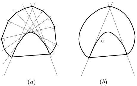
(a) (b)
Figure 1: Two examples of invariant wedges and several tangent subspaces as seen on the unit sphere inR
3
where
Ni,j,k ={n∈R
3 :|n|= 1,hn, p
ii ≤ hn, pji= 0≤ hn, pki}. Let
V = cone{v ∈R
3 :|v|= 1,|v−p
i| ≤a, i= 1,2,3}.
Figure 1(a) sketches the set V and several subspaces orthogonal to elements of N, intersected with the unit sphere. For example, n and t represent a normal in N2,1,3 and its orthogonal subspace. As n varies within N2,1,3, t varies over the planes that pass through 0 and p1 and between p2 and p3.
Proposition 5.1 Let D be any domain satisfying Condition 2.1 with a corresponding set N
as in (21), or any subset of it. Then V is an invariant wedge for D, and the conclusions of Theorem 3.1 are valid.
Proof: The elementary details are omitted. Letvsatisfy|v|= 1,|v−pi| ≤a,i= 1,2,3 and let nbe inN1,2,3. We will first show that π
nv ∈V. Letm1,2 be a normal to the plane generated by p1 and p2 and such that hm1,2, p3i>0. Define similarlym2,3 with the condition hm2,3, p1i>0. Then it is easy to show that the following condition is sufficient: (1) z = πnv
|πnv| −p2 satisfies
|z−p2| ≤ a, (2) hm1,2, zi ≥0, and (3) hm2,3, zi ≥ 0. This condition can be verified by direct calculation. A similar argument holds for the other setsNi,j,k.
The symmetry of the (pi) in the last example is not necessary and we have assumed it only for the ease of presentation. We describe more examples without proof. Figure 1(b) shows a set of tangential subspaces and a corresponding invariant wedge. The subspaces all pass through eitherq1 orq2. Figure 2(a) depicts a different structure. Figure 2(b) shows a continuous version of this structure. In particular, any tangent plane to ∂D (at a smooth portion) will be parallel to a plane that is tangential to the curve cand passes though the origin.
In the rest of this section, we prove a result needed in the proof of Lemma 2.1.
Lemma 5.1 Let V ⊂R
d be a convex closed set and for ǫ >0 let Vǫ be defined as in (5). Then
c
(a) (b)
Figure 2: More examples in dimension three
Proof:By convexity ofV, for anyu∈Vc there exists a uniquev∈∂V for whichǫ= dist(u, V) =
|u−v|, and moreoverm(u) = (v−u)/ǫ.
Let nowu∈Vc andσ >0 be given. We will show that there exists an η >0 such that u′ ∈Vc and |u −u′| < η imply |m(u) −m(u′)| < σ. Let ǫ = dist(u, V) and v ∈ ∂V be such that
|u−v| =ǫ. For u′ ∈ Vc let v′ ∈∂V be such that |u′−v′|= dist(u′, V). Choose α such that
˜
u=u′+αm(u′) will satisfy dist(˜u, V) =ǫ. Note that dist(˜u, V) =|u˜−v′|and as a consequence m(˜u) =m(u′).
We claim that the following inequality must hold
|v−v′| ≤ |u−u˜|. (22)
Indeed, the fact that|u−v|<|u−(λv+(1−λ)v′)|for anyλ∈(0,1) implies thathu−v, v−v′i ≥0.
Similarly, hu˜−v′, v′−vi ≥0. Hence follows (22). One now has that
|m(u)−m(u′)| ≤ |u−u˜|+|v−v′| ǫ
≤ 2|uǫ−u˜|
≤ 4|u−u′|
ǫ .
The last inequality follows from |u′ −u˜|= |dist(u′, V)−dist(u, V)| ≤ |u′ −u|. One may now
takeη =σǫ/4 and conclude that|m(u)−m(u′)|< σif|u−u′|< η.
Acknowledgments. I wish to thank Siva Athreya for introducing me to the problem. I am grateful also to Yehuda Pinchover for helpful discussions and suggestions, and to Krzysztof Burdzy, Min Kang, Gary Lieberman, Ross Pinsky and Ofer Zeitouni for their valuable comments.
References
[2] R. F. Bass.Probabilistic Techniques in Analysis,Series of Prob. Appl. (1995)
[3] R. F. Bass and K. Burdzy.Fiber Brownian motion and the “hot spots” problem,Duke Math. J. 105 (2000), no. 1, 25–58.
[4] R. F. Bass and P. Hsu.Some potential theory for reflecting Brownian motion in H¨older and Lipschitz domains,Ann. Prob. Vol. 19 No. 2 486–508 (1991)
[5] K. Burdzy and W. Werner.A counterexample to the “hot spots” conjecture,Ann. Math. 149 309–317 (1999)
[6] M. Cranston and Y. Le Jan. Noncoalescence for the Skorohod equation in a convex domain ofR
2,
Probab. Theory Related Fields 87, 241–252 (1990)
[7] E. B. Davies.Heat Kernels and Spectral Theory, Cambridge University Press, 1989.
[8] P. Dupuis and H. Ishii. On Lipschitz continuity of the solution mapping to the Skorokhod problem, with applications, Stochastics and Stochastics Reports, Vol. 35, pp. 31–62 (1991)
[9] P. Dupuis and K. Ramanan. Convex duality and the Skorokhod Problem. I, II, Probab. Theory
Related Fields 115 (1999), no. 2, 153–195, 197–236.
[10] D. Jerison and N. Nadirashvili.The “hot spots” conjecture for domains with two axes of symmetry, J. Amer. Math. Soc. 13 (2000), no. 4, 741–772
[11] B. Kawohl.Rearrangements and Convexity of Level Sets in PDE, Lecture Notes in Mathematics,
Vol. 1150 (1985)
[12] M. A. Krasnosel’skij, Je. A. Lifshits and A. V. Sobolev. Positive Linear Systes: The Method of Positive Operators,Sigma Series in Appl. Math. Vol. 5 (1989)
[13] O. A. Ladyˇzenskaja, V. A. Solonnikov and N. N. Ural’ceva. Linear and Quasilinear Equations of Parabolic TypeTransl. Math. Monogr., Vol. 23, AMS, Providence (1968)
[14] P. L. Lions and A. S. Sznitman.Stochastic differential equations with reflecting boundary conditions, Comm. Pure appl. Math. Vol. 37, 511–537 (1984)
[15] D. Lupo and A. M. Micheletti.On the persistence of the multiplicity of eigenvalues for some varia-tional elliptic operator depending on the domain,J. Math. Anal. Appl. 193 no. 3 990–1002 (1995)