www.elsevier.nl / locate / econbase
Taxpayer response to an increased probability of audit:
evidence from a controlled experiment in Minnesota
a ,* b c
Joel Slemrod , Marsha Blumenthal , Charles Christian a
The University of Michigan Business School, 701 Tappan Street, Room A2120D, Ann Arbor,
MI48109-1234, USA b
University of St. Thomas, St. Paul, MN 55105, USA
c
Arizona State University, Tempe, AZ 85287-3606, USA
Received 1 April 1999; received in revised form 1 September 1999; accepted 2 September 1999
Abstract
In 1995 a group of 1724 randomly selected Minnesota taxpayers was informed by letter that the returns they were about to file would be ‘closely examined’. Compared to a control group that did not receive this letter, low and middle-income taxpayers in the treatment group on average increased tax payments compared to the previous year, which we interpret as indicating the presence of noncompliance. The effect was much stronger for those with more opportunity to evade; in fact, the difference in differences is not statistically significant for those who do not have self-employment or farm income, and do not pay estimated tax. Surprisingly, however, the reported tax liability of the high income treatment
group fell sharply relative to the control group. 2001 Elsevier Science B.V. All rights
reserved.
Keywords: Taxation; Evasion; Experiment
JEL classification: H26; C93
1. Introduction
Tax evasion is a quantitatively significant phenomenon that affects the equity, efficiency, and simplicity of a tax system. For example, because most taxpayers
*Corresponding author. Tel.:11-734-936-3914; fax:11-734-763-4032.
E-mail address: [email protected] (J. Slemrod).
456 J. Slemrod et al. / Journal of Public Economics 79 (2001) 455 –483
will not voluntarily pay taxes in the absence of an enforcement mechanism, the potential for evasion must be considered in the design of tax structure. The phenomenon of evasion also raises challenging questions about the appropriate design of the tax enforcement agency itself: how many resources should be devoted to auditing suspected evaders; how should these resources be allocated across classes of taxpayers; how many resources should be devoted to taxpayer assistance rather than monitoring; can evasion be reduced by appeals to taxpayers’ conscience, or sense of duty?
The formulation of informed policy in these areas has been hampered by a paucity of reliable quantitative information on the likely effects of these alternative policies. The critical information is to what extent taxpayers would alter their compliance behavior in response to the set of possible policy alternatives. As we will argue below, existing empirical work — statistical, and experimental — is plagued by serious enough problems that the findings are subject to considerable doubt.
In this paper we discuss the results of a controlled experiment regarding income tax compliance that is not subject to the biases of other approaches to investigating the impact of alternative tax enforcement policies. In 1995 the Minnesota Department of Revenue conducted a series of income tax compliance experiments to test alternative strategies for improving tax administration and increasing
1
voluntary compliance. Approximately 47,000 Minnesota taxpayers who filed 1993 income tax returns were selected at random for one of five experimental ‘treatments’ that were administered at the beginning of the filing season for 1994 returns. One treatment group was offered enhanced taxpayer assistance, including help with their federal return that was not previously offered by the State. Another received a redesigned Minnesota income tax return form with additional line items for reporting Minnesota adjustments to federal taxable income. Two additional large groups received ‘educational’ letters from the Commissioner of Revenue that appealed to their sense of equity or to their sense of social norms.
In this paper we focus on an experiment designed to learn about the impact of an increased probability of audit. A group of 1724 randomly selected taxpayers was informed by letter that the returns they were about to file, both state and
federal, would be ‘closely examined’. This is an especially interesting experiment
1
because, under certain assumptions, the response of taxpayers provides an estimate of the extent of tax evasion.
The Department of Revenue sampled data from 1993 Minnesota income tax returns as they were filed during calendar year 1994. The 1993 data were matched to corresponding data from the 1994 returns of the same taxpayers after the experimental intervention. These 2 years of data from the same taxpayers enable comparisons of changes in reported income, deductions, and tax liability between those taxpayers who received the treatments and similar groups of taxpayers who were not subject to any treatment (the control groups). Data from the 1993 and 1994 federal tax returns of the subjects of the audit experiment, both those who received the treatments and those who served as controls, were also made available. Data from the federal income tax returns include far more detail than the state tax returns because the Minnesota state income tax return is based on federal taxable income.
We find that the treatment effect varies depending on the level of income. Low and middle income taxpayers in the treatment group increased reported tax between 1993 and 1994 relative to the control group, which we interpret as indicating the presence of noncompliance. The effect was much stronger for those with more ‘opportunity’ to evade, as measured by their source of income. Surprisingly, however, the reported tax liability of the high income treatment group fell sharply in 1994 relative to the control group. We suggest a model that can explain this apparently perverse response.
2. Theory
Suppose that the true tax base is not costlessly observable to the tax collection agency, although known to the taxpayer. Then, under certain circumstances, the taxpayer may be tempted to report a taxable income below the true value. In the seminal formulation of Allingham and Sandmo (1972) (henceforth A-S), what might deter an individual from income tax evasion is a fixed probability ( p) that any taxable income understatement will be detected and subjected to a penalty (u)
2
over and above payment of the true tax liability itself.
In the A-S model, all real decisions, and therefore taxable income ( y), are held fixed; only the taxpayer’s report is chosen. The taxpayer chooses a report (x), where x#y, and thus an amount of evasion y2x, in order to maximize
EU5(12p)U(n 1t( y2x))1pU(n 2 u( y2x)), (1)
where n is true after-tax income, y(12t), t being the rate of (proportional)
2
458 J. Slemrod et al. / Journal of Public Economics 79 (2001) 455 –483
income tax. The first-order condition for an optimal interior value of x is simply
U9( y ) /U9( y )5(12p)t /pu, where y and y are income in the audited and
A U A U
3
unaudited state, respectively. Most important for our purposes, the model predicts that regardless of preferences, increases in p will decrease evasion: if p equals one,
any rational taxpayer will report his or her true income.
This model also predicts that a risk-neutral individual would either, if the evasion has a positive expected payoff, remit no tax at all, or if evasion had a negative expected payoff, do no evasion. As discussed in Yitzhaki (1987), the corner solution aspect of the model is eliminated however, if the probability of detection is an increasing function of the amount of evasion. In this case the
4
model’s predictions depend on the precise relationship between p and evasion. Expected income is simply
EY5(12p[x])(n 1t( y2x))1p[x](n 2 u( y2x)). (2)
If p9;≠p /≠x is zero, then the risk-neutral taxpayer evades an unlimited amount as
long as it has positive expected value, i.e. when (12p)t2pu .0. When p9 is
negative, so that the probability of audit falls with an increased report, the first-order condition becomes
(12p)t2pu 5 2p9(u 1t)( y2x). (3)
In this case, evasion will be constrained by the fact that p increases to offset what would otherwise be an increase in expected income.
3. Empirical studies of tax evasion
3.1. What is known
Ascertaining the extent, characteristics, and determinants of evasion
immedi-3
Yitzhaki (1974) amended the A-S formulation to allow the penalty for discovered evasion to depend on the tax (not, as in A-S, the income) understatement, as more accurately reflects practice in many countries. In this case, the maximand becomes (12p)U(n 1t( y2x))1pU(n 2 ut( y2x)). This is
critical for understanding the impact on evasion for a change in t, because it means that the tax rate has no effect on the terms of the tax evasion gamble; as t rises, the payoff to a successful understatement of a dollar rises, but the cost of a detected understatement rises proportionately. It is not critical for understanding the impact of changes in p, which is our focus.
4
The endogenous probability of detection can of course be applied to the case of a risk-averse taxpayer. In this case, at the margin the gain in expected value is offset by a combination of increased risk-bearing and an increased probability of detection. Cremer and Gahvari (1994) generalize this notion by introducing what they call a ‘concealment technology’, which takes the form p(e, e /y, m), where e is the amount of income not reported ( y2x in the notation used above), e /y is the ratio of
ately runs into two problems — one conceptual and one empirical. The conceptual problem is that, although one can assert that legality is the dividing line between evasion and avoidance, in practice the line is often blurry; sometimes the law itself is unclear, sometimes it is clear but not known to the taxpayer, sometimes the law is clear but the administration effectively ignores a particular transaction or activity.
The other difficulty is that, by its nature, tax evasion is not easy to measure — merely asking just won’t do. The most reliable source of information about tax compliance concerns the US federal income tax, and exists because of the IRS’s Taxpayer Compliance Measurement Program (TCMP). Under this program, approximately every 3 years from 1965 until 1988 the IRS conducted a program of intensive audits on a large stratified random sample of tax returns, using the results to develop a formula used to inform the selection of returns for regular audits. The TCMP data consist of line-by-line information about what the taxpayer reported, and what the examiner concluded was correct.
Analysis of the TCMP data suggests that the tax gap is about 17% of true tax liability. However, much of this tax gap refers to nonfilers and to estimates of noncompliance undetected by the TCMP; the TCMP-detected rate of noncom-pliance is 7.3%. The extent of evasion varies widely across types of gross income and deductions; for example, the 1988 TCMP indicates that the voluntary reporting percentage was 99.5% for wages and salaries, but only 41.4% for self-employment income (Schedule C). The fraction of income that is underre-ported declines with income. For example, Christian (1994) reports that, in 1988, taxpayers with (audit-adjusted) incomes over $100,000 on average reported 96.6% of their true incomes to the IRS, compared to 85.9% for those with incomes under
5
$25,000. Finally, within any group defined by income, age, or other demographic category, there are some who evade, some who do not, and even some who (presumably inadvertently) overstate tax liability. For example, of middle-income (income between $50,000 and $100,000) taxpayers in 1988, 60% understated tax, 26% reported correctly, and 14% overstated tax (Christian, 1994, p. 39).
Empirical attempts to establish more systematically how compliance responds to aspects of the tax environment have met with limited success, primarily due to inherent data problems. Clotfelter (1983) and Feinstein (1991) analyzed the TCMP data to investigate how noncompliance responded to changes in the environment, focusing on the impact of the tax rate. Neither analysis investigated the impact of the probability of detection on noncompliance. Clotfelter argued that calculated arrest and conviction rates would probably not correspond closely to the
5
460 J. Slemrod et al. / Journal of Public Economics 79 (2001) 455 –483
perceptions of would-be evaders and would, in any event, not be exogenous; his
6
regressions were carried out separately by audit class.
Dubin et al. (1990) make use of state-level time-series cross-section data from 1977 through 1985 to investigate the impact of audit rates and tax rates on tax compliance. They do not, though, have a direct measure of noncompliance, but instead use tax collections per return filed and returns filed per capita as (inverse) measures of noncompliance. They conclude that the continual decline in the audit rate over this period caused a significant decline in IRS collections. Note, though, that their measure of noncompliance will be affected by changes in the tax law as well as other changes in the economy, and their measure of the probability of detection is subject to the same endogeneity problems as the cross-sectional analyses.
3.2. The promise of a controlled experiment
A generic problem with both the time-series and cross-sectional studies is that the probability of detection ( p) is difficult to measure and, furthermore, its variation may not be random but rather a response by the IRS to perceived variations in the extent of evasion or effectiveness of enforcement. The virtue of a controlled experiment is that the source of variation in p is unambiguous and is certainly not a response to the environment. Controlled experiments have been used fairly extensively since the late 1960s to investigate a wide range of economics issues; their strengths and weaknesses have been nicely surveyed by Burtless (1995) and Heckman and Smith (1995). Their applicability to tax compliance research was discussed in a paper by Boruch (1989) for the National Research Council’s Panel on Taxpayer Compliance Research, which recom-mended that the IRS and external researchers collaborate to expand the use of field experiments to analyze the compliance effects of innovations in tax administration (Roth et al., 1989, p. 229).
One early example of this approach is that of Schwartz and Orleans (1967), who contacted randomly selected groups of taxpayers and asked questions that ‘emphasized the severity of sanctions available to the government and the likelihood that tax violators would be apprehended’ (the sanction group). Another group was asked questions focusing on moral reasons for compliance (the conscience group), a ‘placebo’ group was asked basic interview questions, and a fourth group served as an ‘untreated’ control. The empirical analysis was based on the change between 1961 and 1962 in reported AGI, total deductions, and income tax after credits. For AGI and tax after credits, only the ‘conscience’ group reported a larger increase in tax than the ‘placebo’ or ‘untreated’ control groups.
6
Contrary to expectation, the ‘sanction’ group reported a larger increase in total deductions than the ‘placebo’ group. The authors speculate that subjects may have responded as if thinking, ‘You may beat me into admitting higher income, but I’ll find a way of getting it back’.
The present experiment differs fundamentally from Schwartz and Orleans because taxpayers were contacted by the taxing authority rather than the experimenters, and they were notified that their return would be ‘closely examined’. Both make the present methods more appropriate for testing for the effects of enforcement actions on reporting behavior.
4. Design of the experiments
4.1. Sample design
The subjects for this experiment were selected randomly, subject to certain restrictions. Sampled were full-year 1993 Minnesota residents who filed Minnesota tax returns in 1994 for the 1993 tax year, and whose 1993 return was processed by the Minnesota Department of Revenue by the end of September, 1994. No amended returns were included; and matching federal income tax data had to be available for the taxpayers. About 1,853,000 Minnesota taxpayers met these conditions.
The portion of the sample used for the final analysis consisted of taxpayers whose 1994 Minnesota tax returns were filed and processed by the Department of Revenue by the end of December, 1995, or for whom federal tax returns were filed during 1995. Some loss of taxpayers in the sample was undoubtedly caused by taxpayers moving out of state or having too little income to file a 1994 return, among other possibilities. The December processing date, however, allowed us to include most of the taxpayers who might have filed late or requested an extension in 1995, perhaps as a result of the experimental treatment.
The sample was stratified by income and by a set of characteristics we refer to as opportunity. There were three stratifications by 1993 income: low-income, with AGI less than $10,000; middle-income, with AGI between $10,000 and $100,000; and high-income, with AGI over $100,000.
Previous research on tax evasion points to several factors associated with evasion, including income not subject to withholding tax and income from a sole proprietorship. The ‘high-opportunity’ group was a random sample from taxpayers who filed a federal Schedule C or F (indicating business or farm income) in 1993
and who paid Minnesota estimated tax. A Minnesota taxpayer is required to file
462 J. Slemrod et al. / Journal of Public Economics 79 (2001) 455 –483
Low income / low opportunity 449,017 0.10% 460 976.1 Low income / high opportunity 2120 2.69% 57 37.2 Medium income / low opportunity 1,290,233 0.04% 567 2275.5 Medium income / high opportunity 50,920 0.84% 429 118.7 High income / low opportunity 52,093 0.22% 114 457.0 High income / high opportunity 8456 1.03% 87 97.2
Total 1,852,839 1714
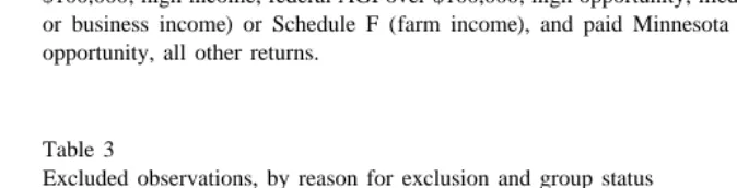
a
Low income, federal AGI less than $10,000; middle income, federal AGI from $10,000 to $100,000; high income, federal AGI over $100,000; high opportunity, filed a federal Schedule C (trade or business income) or Schedule F (farm income), and paid Minnesota estimated tax in 1993; low opportunity, all other returns.
7
but expected to have little reported income from their businesses. Taxpayers not in the high-opportunity category are referred to as low-opportunity.
The population count, sampling rate, and the resulting sample frequency for each stratum are presented for the treatment group in Table 1 and for the control
8
group in Table 2. Table 3 documents the further reduction in the sample by the elimination of returns (1) changing to, or from, married filing jointly, (2) filing for a different tax year, (3) not filing a 1994 tax return, or (4) having no positive
9
income. This produced a working sample of 22,368 returns.
4.2. Experimental treatment
The treatment group received a letter by first-class mail from the Commissioner
10
of Revenue in January of 1995. Note that this treatment was administered after the tax year, and at the beginning of the filing season. Thus, with a few exceptions (such as contributions to IRAs or Keoghs) it could not have affected non-reporting
7
An advantage of a sample based on estimated-tax payers is the possibility of tailoring interventions for this group in the future if the experiment proved a success, because these taxpayers are involved with the department throughout the year. The low-opportunity group selected to represent the general population may provide valuable information about what approach to compliance works best with people who rarely would be the target of an audit.
8
The control group from the ‘audit’ experiment was combined with the control group from the ‘appeal to conscience’ experiment to increase precision. Both were randomly selected, and neither was contacted by the Department of Revenue during the experiment.
9
We also excluded a number of returns for which there was a single 1993 return associated with two 1994 returns, presumably due to divorce.
10
Table 2
a Control group sample selection
Stratum Population Sampling n Weight
rate
Low income / low opportunity 449,017 1.30% 5821 77.1
Low income / high opportunity 2120 6.56% 139 15.3
Medium income / low opportunity 1,290,233 1.15% 14,817 87.1 Medium income / high opportunity 50,920 2.76% 1403 36.3 High income / low opportunity 52,093 1.42% 739 70.5 High income / high opportunity 8456 3.15% 266 31.8
Total 1,852,839 23,185
a
Low income, federal AGI less than $10,000; middle income, federal AGI from $10,000 to $100,000; high income, federal AGI over $100,000; high opportunity, filed a federal Schedule C (trade or business income) or Schedule F (farm income), and paid Minnesota estimated tax in 1993; low opportunity, all other returns.
Table 3
Excluded observations, by reason for exclusion and group status
Sample selection Treatment Control Total
1993 filers 1714 23,185 24,899
Changed filing status 254 23.2% 2973 24.2% 21027 Filed for different tax year 21 20.1% 27 0.0% 28 Did not file 1994 federal return 2122 27.1% 21370 25.9% 21492
No positive income 0.0% 24 0.0% 24
Total 1537 20,831 22,368
11
behavior with tax consequences. The taxpayers were told: (1) that they had been selected at random to be part of a study ‘that will increase the number of taxpayers whose 1994 individual income tax returns are closely examined’; (2) that both their state and federal tax returns for the 1994 tax year would be closely examined by the Minnesota Department of Revenue; (3) that they will be contacted about any discrepancies; and (4) that if any ‘irregularities’ were found, their returns filed
12
in 1994 as well as prior years might be reviewed, as provided by law. The
11
This aspect of the experiment is consistent with the Allingham and Sandmo (1972) assumption of a fixed ‘true’ taxable income.
12
464 J. Slemrod et al. / Journal of Public Economics 79 (2001) 455 –483
taxpayers were given department phone numbers to call for information and
13
assistance with their taxes.
To what extent the receipt of this letter corresponds to a ‘p equals one’ experiment is an open question. Some taxpayers may believe that some aspects of noncompliance would not be detected by an ‘examination’. Others might have believed that this was an idle, or incredible, threat. In the concluding section we return to these issues in light of the results, which we discuss next.
5. Results
5.1. Measuring compliance
According to the IRS, compliance has three parts: accurate reporting, timely
14
filing, and timely paying; this paper focuses solely on the first. We had no access to the results of audits as a measure of accuracy. Instead, to measure accurate reporting we investigate the response of three measures of reported income and tax liability: federal taxable income, federal tax after credits, and Minnesota tax
15
liability. We examine the changes in reported tax liability (or taxable income) between 1993 and 1994 for the treatment group relative to the control group: a
16,17
difference-in-difference methodology.
If the 1993 to 1994 change for the treatment group was different than the
13
The pertinent text of the letter was as follows: Dear Taxpayer:
This year we are doing a study that will increase the number of taxpayers whose 1994 individual income tax returns are closely examined by the Minnesota Department of Revenue. You have been selected at random from a list of all Minnesota taxpayers to be in this study.
The examination of your 1994 tax returns will include both your state and federal returns. After a close review of your returns, we may write to you for additional information about them or arrange a face-to-face audit. If the examination of your 1994 returns finds any irregularities, we may also review tax returns you filed in prior years, as provided by law.
When you prepare your 1994 return, or give information to your tax preparer, please be very careful to report all your income and take only the deductions to which you are entitled. Remember to attach a copy of your federal return to your state return.
The Minnesota Department of Revenue tries to help taxpayers comply with the law. If you have questions about your Minnesota income tax return, please call us at these numbers.
14
There was no statistically significant difference in the date filed (technically, the date received by the IRS) between the control and treatment groups. For evidence on the determinants of filing date, see Slemrod et al. (1997).
15
We have access only to unaudited returns, so we cannot directly assess, for example, the impact of the treatment on the ‘accuracy’ of tax returns.
16
1993 values are adjusted for inflation, so all measures are in 1994 dollars. 17
average change for the control group, we infer that the treatment had an effect on taxpayer compliance behavior, provided that the difference between groups was large enough to be statistically significant. Although we cannot verify that changes in reported tax liability or taxable income were due to changed compliance behavior, because subjects were randomly assigned to treatment and control groups, this inference seems unassailable. We do not have access to the results of the ‘close examination’ given to the returns from the treatment group, nor to any audit results more generally, so a more direct (although still imperfect) measure of non-compliance is not available.
5.2. Mean difference in differences: low- and middle-income taxpayers
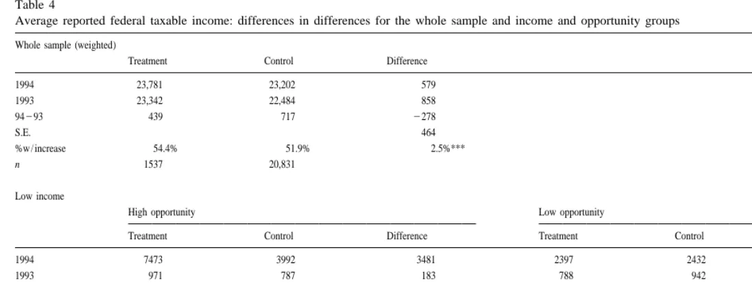
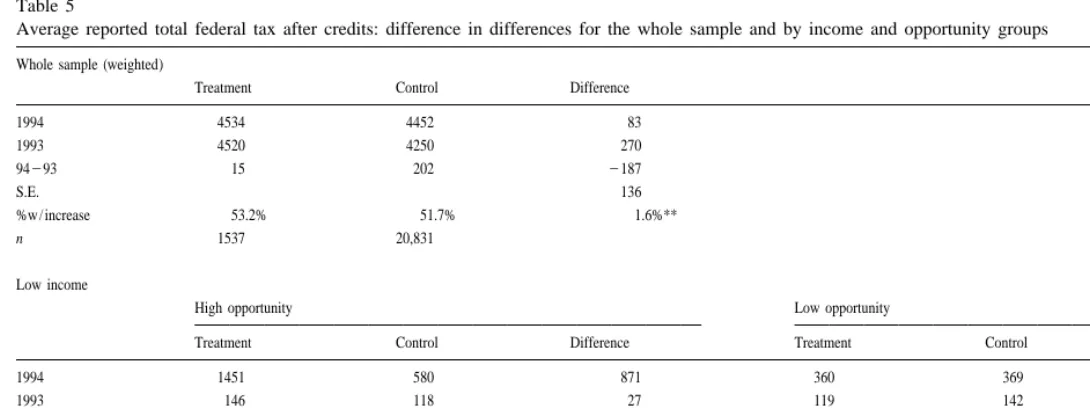
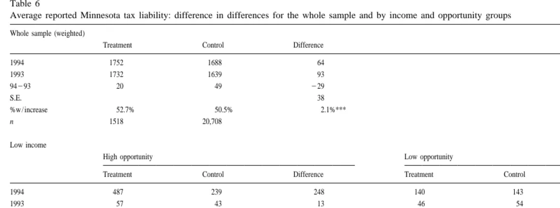
Much of the interest, and puzzles, regarding the results are apparent in the tabulation of means presented in Tables 4–6, which concern, respectively, federal taxable income, federal tax after credits, and Minnesota income tax liability. Because for the most part Tables 4–6 tell a similar story, we focus here on Table 5. It lists the mean of federal tax liability after credits separately for the treatment and control groups for 1993 and 1994, as well as the absolute mean change between 1993 and 1994. The last column shows the difference between the treatment and control group means for these four variables. The fifth row of data is a non-parametric measure of the behavioral response, the fraction of tax returns which showed an increase in the (inflation-adjusted) value between 1993 and
18
1994.
Consider first the low and middle-income groups. Notice first that the 1993 means for the control and treatment groups are very close, attesting to the randomness of the sample selection procedures. Among both the low- and middle-income strata, the audit notice apparently had a very large impact on the high-opportunity taxpayers. The average difference-in-difference federal tax liability was $676 for the middle-income group. This compares to an average $5606 of 1994 tax liability for the control group, amounting to a 12.1% increase in tax. For the lower-income, high-opportunity group the apparent treatment effect is even more striking; the difference-in-difference was $843, compared to 1994 tax liability for the control group of $580, amounting to a 145.3% increase. However, only the middle-income result was statistically significant at a 10% level. Qualitatively the same results apply if we look at the fraction of taxpayers for whom real tax payments increased from 1993 to 1994 — a larger treatment effect among the high-opportunity taxpayers compared to the low-opportunity taxpayers.
18
466
J.
Slemrod
et
al
.
/
Journal
of
Public
Economics
79
(2001
)
455
–
483
Table 4
Average reported federal taxable income: differences in differences for the whole sample and income and opportunity groups Whole sample (weighted)
Treatment Control Difference
1994 23,781 23,202 579
1993 23,342 22,484 858
94293 439 717 2278
S.E. 464
%w / increase 54.4% 51.9% 2.5%***
n 1537 20,831
Low income
High opportunity Low opportunity
Treatment Control Difference Treatment Control Difference
1994 7473 3992 3481 2397 2432 235
1993 971 787 183 788 942 2154**
94293 6502 3204 3298 1609 1490 119
S.E. 2718 189
%w / increase 65.4% 51.2% 14.2%* 52.2% 50.2% 2.0%
Slemrod
et
al
.
/
Journal
of
Public
Economics
79
(2001
)
455
–
483
467
High opportunity Low opportunity
Treatment Control Difference Treatment Control Difference
1994 33,280 31,191 2089 24,316 23,669 646
1993 29,735 29,652 83 23,355 23,172 183
94293 3546 1539 2007 960 497 463
S.E. 1494 466
%w / increase 57.2% 53.1% 4.1% 56.0% 52.8% 3.2%
n 397 1318 520 13,636
High income
High opportunity Low opportunity
Treatment Control Difference Treatment Control Difference
1994 143,170 163,015 219,845 146,198 145,161 1037
1993 176,683 150,865 25,818 164,919 147,819 17,099
94293 233,513 12,150 245,663*** 218,721 22659 216,063
S.E. 17,394 10,455
%w / increase 37.5% 42.2% 24.7% 32.7% 43.6% 210.9%**
n 80 244 107 681
a
*P,0.10; **P,0.05; ***P,0.01. Low income, federal AGI less than $10,000; middle income, federal AGI from $10,000 to $100,000; high income, federal
468
J.
Slemrod
et
al
.
/
Journal
of
Public
Economics
79
(2001
)
455
–
483
Table 5
Average reported total federal tax after credits: difference in differences for the whole sample and by income and opportunity groups Whole sample (weighted)
Treatment Control Difference
1994 4534 4452 83
1993 4520 4250 270
94293 15 202 2187
S.E. 136
%w / increase 53.2% 51.7% 1.6%**
n 1537 20,831
Low income
High opportunity Low opportunity
Treatment Control Difference Treatment Control Difference
1994 1451 580 871 360 369 210
1993 146 118 27 119 142 222**
94293 1305 462 843 240 228 13
S.E. 726 29
%w / increase 63.5% 51.2% 12.2% 50.1% 49.2% 0.9%
Slemrod
et
al
.
/
Journal
of
Public
Economics
79
(2001
)
455
–
483
469
High opportunity Low opportunity
Treatment Control Difference Treatment Control Difference
1994 6201 5606 595 4065 3992 73
1993 5082 5162 280 3818 3837 219
94293 1120 444 676* 247 155 92
S.E. 394 113
%w / increase 56.7% 53.3% 3.4% 55.0% 52.8% 2.2%
n 397 1318 520 13,636
High income
High opportunity Low opportunity
Treatment Control Difference Treatment Control Difference
1994 38,703 45,597 26894 40,577 40,339 239
1993 49,637 40,671 8966 47,190 40,194 6996
94293 210,934 4925 215,860*** 26613 144 26757*
S.E. 6054 3854
%w / increase 36.3% 42.2% 26.0% 33.6% 43.6% 210.0%
n 80 244 107 681
a
*P,0.10; **P,0.05; ***P,0.01. Low income, federal AGI less than $10,000; middle income, federal AGI from $10,000 to $100,000; high income, federal
470
J.
Slemrod
et
al
.
/
Journal
of
Public
Economics
79
(2001
)
455
–
483
Table 6
Average reported Minnesota tax liability: difference in differences for the whole sample and by income and opportunity groups Whole sample (weighted)
Treatment Control Difference
1994 1752 1688 64
1993 1732 1639 93
94293 20 49 229
S.E. 38
%w / increase 52.7% 50.5% 2.1%***
n 1518 20,708
Low income
High opportunity Low opportunity
Treatment Control Difference Treatment Control Difference
1994 487 239 248 140 143 23
1993 57 43 13 46 54 29*
94293 430 195 234 94 89 5
S.E. 208 11
%w / increase 59.6% 48.0% 11.6% 48.3% 47.3% 0.9%
Slemrod
et
al
.
/
Journal
of
Public
Economics
79
(2001
)
455
–
483
471
High opportunity Low opportunity
Treatment Control Difference Treatment Control Difference
1994 2370 2201 169 1702 1649 53
1993 2093 2093 0 1627 1609 18
94293 277 108 169 75 41 35
S.E. 121 37
%w / increase 56.6% 51.7% 4.9%* 54.8% 51.9% 3.0%
n 394 1313 516 13,582
High income
High opportunity Low opportunity
Treatment Control Difference Treatment Control Difference
1994 12,397 13,825 21428 12,870 12,274 596
1993 15,854 12,798 3056 14,448 12,541 1907
94293 23457 1027 24484*** 21578 2267 21311
S.E. 1540 804
%w / increase 36.4% 41.8% 25.4% 33.0% 42.9% 29.8%*
n 77 244 106 679
a
472
J.
Slemrod
et
al
.
/
Journal
of
Public
Economics
79
(2001
)
455
–
483
Table 7
1993–1994 change in components of income for treatment and control groups, by income and opportunity group Whole sample (weighted)
n Treatment n Control Difference S.E.
Federal taxable income 1537 439.11 20,831 717.49 2278.38 464.74
Wages and salaries 1537 2207.71 20,831 519.59 2727.31** 340.98 Interest 1537 2137.12 20,831 246.42 290.70** 55.07 Dividends 1537 6.21 20,831 3.07 3.14 21.49 Net Schedule C income 1537 166.76 20,831 87.16 79.60 100.76 Capital gains 1537 168.40 20,831 2254.94 423.34* 308.33 Other gains 1537 270.34 20,831 215.94 254.40 77.28 Other income 1537 38.64 3073 240.37 79.02 97.79 Total adjustments 1537 219.57 20,831 221.12 1.55 19.37 Itemized deductions 1537 2386.92 20,831 2203.70 2183.22* 138.80
Low income
High opportunity Low opportunity
n Treatment n Control Difference S.E. n Treatment n Control Difference S.E.
Federal taxable income 52 6501.82 123 3204.04 3297.78 2718.70 381 1609.02 4829 1490.20 118.82 189.51
J.
Slemrod
et
al
.
/
Journal
of
Public
Economics
79
(2001
)
455
–
483
473
High opportunity Low opportunity
n Treatment n Control Difference S.E. n Treatment n Control Difference S.E.
Federal taxable income 397 3545.69 1318 1539.14 2006.55 1494.08 520 960.33 13,636 497.01 463.32 466.12
Wages and salaries 397 1569.22 1318 772.35 796.87 728.40 520 226.31 13,636 214.14 2240.45 349.49 Interest 397 2168.73 1318 2278.75 110.03 103.60 520 2200.50 13,646 256.78 2143.72** 58.35 Dividends 397 18.23 1318 88.70 270.47 72.06 520 21.52 13,636 218.74 40.25*** 13.44 Net Schedule C income 397 26.93 1318 2672.60 665.67 925.83 520 194.73 13,636 81.67 113.06 116.56 Capital gains 397 659.25 1318 2368.64 1027.89 966.97 520 191.17 13,636 270.10 261.27 236.65 Other gains 397 280.73 1318 295.97 215.24 461.81 520 271.61 13,636 236.68 234.93 102.44 Other income 397 13.52 798 81.33 267.81 113.39 520 35.09 1045 29.12 44.21 59.50 Total adjustments 397 2186.87 1318 2271.50 84.63 120.56 520 213.07 13,636 217.67 4.60 25.82 Itemized deductions 397 2502.55 1318 2371.28 2131.26 276.93 520 2452.02 13,636 2194.29 2257.73 176.89
High income
High opportunity Low opportunity
n Treatment n Control Difference S.E. n Treatment n Control Difference S.E.
Federal taxable income 80 233,513.20 244 12,150.02 45,663.22*** 17,395.51 107 218,721.30 681 22658.50 216,062.80 10,505.43
Wages and salaries 80 219,557.83 244 602.02 220,159.85 13,413.07 107 219,344.35 681 22890.87 216,453.48** 7384.87 Interest 80 6145.55 244 233.96 5911.59 5504.27 107 2648.49 681 128.01 2776.50 848.64 Dividends 80 2321.79 244 893.47 21215.26 1657.92 107 2215.31 681 349.09 2564.40 603.64 Net Schedule C income 80 22984.91 244 1039.86 24024.77 7725.09 107 2569.79 681 150.68 2720.47 861.81 Capital gains 80 220,912.61 244 3398.29 224,310.90* 12,473.52 107 2892.96 681 27770.78 10,663.74 8443.18 Other gains 80 2545.27 244 265.18 2810.45 1781.22 107 2657.54 681 2128.17 2529.38 653.55 Other income 80 307.41 153 21344.02 1651.43 1290.18 107 561.19 211 114.48 446.71 1801.26 Total adjustments 80 2906.77 244 2671.18 2235.60 495.99 107 2151.24 681 231.86 2119.38 129.06 Itemized deductions 80 22075.46 244 2813.02 21262.44 25195.23 107 21419.90 681 21948.88 528.98 1706.39
a
474 J. Slemrod et al. / Journal of Public Economics 79 (2001) 455 –483
Although these are striking results, they apply to a small fraction of Minnesota taxpayers — just 53,040 out of 1,852,839, or 2.9%. To get a feel for the potential impact of increased enforcement on aggregate tax liability, we must turn our attention to the ‘low-opportunity’ taxpayers. For the low- and middle-income members of this category, the mean treatment effect is positive, but is of a much smaller magnitude than for the high-opportunity taxpayers. The difference-in-difference averages $92 for the middle-income taxpayers, or 2.3% of the average 1994 tax liability of the control group. For the low-income group the absolute difference-in-differences is only $13, 3.5% of the average 1994 tax liability of the control group. Neither of these differences is different from zero at a high confidence level.
If we aggregate the difference-in-difference estimates for the four groups studied so far, we obtain $161 million, or just under 2% of the total 1994 tax liability of $8.15 billion. This is obviously much lower than the 17% aggregate income tax gap estimated by the IRS, and significantly lower than the TCMP-detected noncompliance of 7.3%.
5.3. Income components
Table 7 presents information about how the components of federal taxable
19
income changed between 1994 and 1993 for the treatment and control groups. For the lower and middle income groups, as expected the predominant response is not in those sources of income that are subject to pervasive information reporting — wages, interest, and dividends. A consistently large identifiable component is capital gains, which are conceivably subject to post-tax-year manipulation through the choice of which shares of a large holding are deemed to have been sold. One might expect that self-employment (Schedule C) income would also be highly manipulable, given the wide discretion in the choice of what qualifies as a business expense. Schedule C income is, in fact, a major component of the apparent treatment effect except for the low-income, high-opportunity group, where the treatment group increased their reported Schedule C income by less than the control group.
5.4. Regression analysis
Table 8 presents the results of a multivariate regression model of the absolute response of the three measures of compliance. This model controls for return characteristics that may better explain the response and improve our ability to test for experimental treatment effects. The regression model also allows for tests of
19
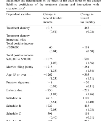
Table 8
Magnitude and determinants of the effect of the audit threat on the change in reported income and tax liability: coefficients of the treatment dummy and interactions with demographic and taxpayer
a characteristics
Dependent variable Change in Change in Change in federal taxable federal Minnesota income tax liability tax liability
Treatment dummy 1018 463 29
(0.51) (0.92) (0.06)
Married filing jointly 21218 2354 253
(1.35) (1.54) (0.74)
Age 65 or over 21262 2395 2116
(1.23) (1.51) (1.42)
Preparer signature 28 220 214
(0.01) (0.11) (0.25)
No. of observations 21,031 21,031 20,895
a
The absolute value of the t-statistics are in parentheses. All specifications include a constant term and the independent variables listed in the table, not interacted with the treatment dummy variable.
interactions between the treatment effect and return characteristics other than income and opportunity. As the analysis of Section 5.3 cannot, it measures the
476 J. Slemrod et al. / Journal of Public Economics 79 (2001) 455 –483
1993 was less than or equal to $100,000, although most of the qualitative results reported below apply to the regression results for the whole sample.
The explanatory variables include dummy variables for ranges of total positive income, marital status, age, the presence of a paid preparer, marginal tax rate, and the presence of various supplemental schedules (Schedules A through F and Schedule ES). To assess the impact of the treatment, we also include a treatment dummy variable, and interactions between the treatment dummy variable and each other regressor.
The regression results indicate that there is a positive treatment effect associated with four indicators of opportunities to evade: the presence of a Schedule A (itemized deductions), Schedule B (interest and dividend receipts), Schedule F
20
(farm income) and a Schedule ES (estimated tax payments). Somewhat surpris-ingly, the presence of a Schedule E, which may include income from partnerships, rents, royalties and trusts, is associated with a negative treatment effect. As an illustration of the quantitative implications, the regression results suggest that a married taxpayer under 65 with total positive income between $50,000 and $100,000 and a marginal tax rate of 28% who prepares his own return, gets a refund, files Schedules A, B and reports estimated tax payments would report $2110 more in federal tax liability if he or she received the treatment letter ($463235411105141519292(16328)). Obviously, this point estimate
de-pends on the return characteristics of the taxpayer. In contrast, a married taxpayer under 65 with less than $20,000 of income, a marginal tax rate of 15%, who self-prepares, takes the standard deduction, files no additional schedules, and gets a refund would, according to these estimates, report about the same federal tax liability upon receiving the treatment letter.
5.5. The ‘perverse’ high-income response
So far we have not discussed the results relating to the high-income taxpayers, who comprise only slightly more than 3% of taxpayers, but who have $2.5 billion, or 30.1% of the federal tax liability. They deserve separate treatment because the results are so strikingly different. First of all, note that the 1993 means for the treatment and control groups are not very close. At a minimum, this testifies to the high variance in reporting behavior among this group. Of most interest is the fact that, compared to the control group, on average the high-income treatment groups exhibit a lower change in reported tax liability from 1993 to 1994. The magnitude of the difference-in-differences is large, amounting to 34.8% of the 1994 control group average tax liability for the high-opportunity group, and 16.8% for the
20
low-opportunity group: for both groups, the difference in means is significant. The unexpected behavior of the high-income groups is also evident in our simple non-parametric analysis — the fraction of taxpayers for whom there was a real increase in tax paid was lower among the treatment groups.
We have pursued two possible explanations for a perverse response of reported
21
income to a notice of examination. The first is that the audit notice letter induced taxpayers to seek out professional tax advisors who, among other things, uncovered legitimate ways to reduce taxable income (even though the tax year had already ended) that the taxpayer had previously been unaware of. A simple version of that hypothesis can be investigated by looking at the change in preparer use. Table 9 documents that the examination notice did increase the percentage of taxpayers (relative to the control group) that made use of professional tax assistance, for high-income taxpayers as well as the other income groups. However, the data on the high-income groups suggests that a shift toward preparer use is unlikely to be a significant part of the story of why the reported income of the treatment group declines, because most of this group was already using a preparer for tax year 1993. This finding does not preclude that taxpayers who used professional tax preparers for tax year 1993 used better or more aggressive tax preparers in 1994, or received different advice in 1994 compared to 1993 from the same preparer.
Another possible explanation relies on an extension of the Allingham–Sandmo model in which taxpayers believe that the probability of audit depends on their
22
report. Our extension relies on the idea that, even upon audit, ‘true’ tax liability is not ascertainable, and the ultimate outcome of an audit depends on the taxpayer’s initial report. To be precise, we are arguing that the expected income upon audit, call it g, is not a monotonically increasing function of x, as in the standard model, but reaches a maximum at some positive level of understatement, where x,y. We return later to what might generate such an outcome. Thus, we
have modified the problem facing a risk-neutral taxpayer to be:
Max EY5(12p[x])(n 1t( y2x))1p[x]( g[x]). (4)
The first-order condition for x now becomes
(12p)t2pg9 5 2p9(v1t( y2x)2g). (5)
21
These explanations presume, of course, that the empirical finding is not spurious. One source of a spurious finding is differential attrition from the sample of the treatment and control groups: perhaps upon receiving the treatment letter, many high-income evaders simply did not file a 1994 return. There is some evidence that the attrition rate is higher for the treatment subset of high-income families, but it is impossible to assess the quantitative impact of this, and we are inclined to believe that this is not an important explanation for our findings.
22
478
J.
Slemrod
et
al
.
/
Journal
of
Public
Economics
79
(2001
)
455
–
483
Table 9
a Practitioner use: difference in differences for the whole sample and by income and opportunity groups Whole sample (weighted)
Treatment Control Difference
1994 53.8% 52.8% 1.0%
1993 50.4% 52.2% 21.8%
94293 3.4% 0.5% 2.9%
S.E. 0.9%
n 1518 20,708
Low income
High opportunity Low opportunity
Treatment Control Difference Treatment Control Difference
1994 76.9% 81.3% 24.4% 46.4% 42.0% 4.4%
1993 75.0% 82.1% 27.1% 45.1% 40.8% 4.3%
94293 1.9% 20.8% 2.7% 1.3% 1.1% 0.2%
S.E. 4.6% 1.6%
Slemrod
et
al
.
/
Journal
of
Public
Economics
79
(2001
)
455
–
483
479
Middle income
High opportunity Low opportunity
Treatment Control Difference Treatment Control Difference
1994 82.2% 82.2% 0.0% 54.1% 53.8% 0.2%
1993 82.2% 84.0% 21.8% 49.8% 53.3% 23.5%
94293 0.0% 21.8% 1.8% 4.3% 0.5% 3.7%
S.E. 1.5% 1.6%
n 394 1313 516 13,582
High income
High opportunity Low opportunity
Treatment Control Difference Treatment Control Difference
1994 88.3% 89.3% 21.0% 70.8% 73.2% 22.4%
1993 88.3% 91.0% 22.7% 67.9% 74.2% 26.3%
94293 0.0% 21.6% 1.6% 2.8% 21.0% 3.9%
S.E. 2.3% 2.5%
n 77 244 106 679
a
480 J. Slemrod et al. / Journal of Public Economics 79 (2001) 455 –483
The question at hand is whether, in the context of this model, it is possible that the optimal report under a ( p51, p9 50) regime could be lower than under a
( p,1, p9 ,0) regime. The answer is yes. Under the former regime, assumed to
characterize the situation in which the treated taxpayers find themselves, the optimum of Eq. (5) reduces to g9 50: in the face of certain audit, one should
simply maximize expected income in the audited state. In the latter (control) situation, the first-order condition (5) is
(12p) p9
]] ]
g9 5 t1 (v1t( y2x)2g). (6)
p p
The first term of the right-hand side of (6) is positive. The second term is negative, because p9 ,0 and v1t( y2x)2g.0 (being audited is a worse state of the
world than not being audited). As long as the second term is larger in absolute value than the first, then at the optimum g9is negative. Thus, given the shape of g,
the optimal value of x for the controls (where g9 ,0) exceeds the optimal value of
x for those that were treated (where g9 50). The intuition is that a certain audit
frees the taxpayer from reporting more income in order to reduce the chance of an audit, and that dominates the fact that the penalty of detected evasion goes from being an event of probability p,1 to one with a probability of one.
We have only now to demonstrate the plausibility that g(x) may reach a maximum at x,y, i.e. that in the face of a certain audit the optimal strategy might
entail some understatement. A simple example where this occurs is if, in the course of an audit, either all evasion is detected and penalized, or none of it is, and
23
if detection is more likely the larger is the amount of understatement. In this case, facing certain audit, a risk-neutral taxpayer maximizes
g(x)5(12q x )(f g v1t( y2x))1q x (f gv2u( y2x)), (7)
which is identical to expression (2) except that now q, the probability of detection and penalty conditioned upon audit, replaces p, and q9 ,0. Clearly, there may be
an optimal x less than y, and there certainly is if q[x5y],t /(t1u).
Some observations about this model are in order. First, it is clear that the change in noncompliance upon the announcement of a certain audit is not, as in the standard A-S model, a measure of noncompliance. Instead, it reveals something about the combined impact of a change in p and a change in p9. There remains the
question of why this effect would dominate only for high-income individuals. The answer must be that members of this group tend to believe that the outcome of the audit process is more manipulable, and the final outcome is more depending on their report, than other taxpayers. It certainly is true that high-income individuals are more likely to have professional assistance with their tax matters and more
23
In an earlier draft we explored another model in which argmax g(x),y, where the taxpayer views
complicated tax affairs, so it is plausible that they also are more likely to have this set of beliefs.
6. Caveats and conclusions
The conclusions to be drawn from this experiment about the magnitude and nature of tax compliance depend critically on how taxpayers interpreted the treatment letters. While the treatments were designed with the purpose of signaling a certain, thorough audit, in actuality they may have had only very limited success in capturing the attention of taxpayers. The phrase ‘we will examine your 1994 tax return very closely’ may have been less threatening than at first blush one might expect. Some people may already believe that their return is being examined ‘very closely’. For such individuals the treatment would have no effect either because they are already deterred or because they have concluded, perhaps incorrectly, that such close inspection is not capable of detecting the type of noncompliance in which they engage. Others may simply not have believed the resource-constrained Minnesota tax enforcement agency could carry out such a large-scale audit program, or that even if they did believe that, may have believed that even such an audit would not uncover their own evasion. Finally, the audit notice indicated that prior returns might also be examined. This element of the treatment may have backfired. Some individuals may have been fearful that if they changed their reporting patterns in 1994 by, for example, reporting income that they had previously not reported, the 1994 report would have given away their history of noncompliance.
These considerations argue against interpreting the difference-in-difference results as a measure of existing noncompliance. However, the results remain relevant as an indicator of the response of taxpayers to an increased enforcement probability, which in practice would be taken more seriously by some taxpayers than others, and whose impact would be conditioned on the taxpayers’ history of noncompliance. This is, after all, the kind of information the Minnesota Depart-ment of Revenue was hoping to glean from this experiDepart-ment.
What, then, have we learned from this randomized, controlled experiment? In terms of methodology, a larger sample size of high-income taxpayers would have
24
increased the certainty with which inferences can be drawn. This is less of a problem with the other income groups, for whom the variability of income reports is much lower. Also, if feasible, a follow-up experiment should begin at the start of the tax year, to allow the audit threat to influence not only reporting decisions,
24
482 J. Slemrod et al. / Journal of Public Economics 79 (2001) 455 –483
25
but also real substitution and avoidance behavior. In the experiment discussed here the treatment was applied only after the tax year was completed, when most behavior with tax consequences (other than IRA or Keogh contributions) had already been carried out.
In summary, we conclude that a heightened threat of examination increases the reported income and tax liability of low- and middle-income taxpayers, especially those that have greater opportunities to evade taxes. The increased tax collections from this group are, though, likely to be fairly small, in this experiment amounting to less than 2% of total tax liability. Moreover, there is reason to suspect that high-income taxpayers may react by reporting even less income than before, based on a perception that an audit will not automatically detect and punish all evasion, and the final outcome may be influenced by the initially reported income. This suggests that a heightened audit threat should be carried out simultaneously with a rethinking of how the audits themselves are carried out.
Acknowledgements
We would like to thank the employees of the Minnesota Department of Revenue — in particular Gerald Bauer, Bob Cline, Steve Coleman, Mary Kim, and Carole Wald — who initiated and executed the experiment described in this paper. The views expressed here are, however, not necessarily shared by the Department or these individuals. Expert research assistance was provided by Jon Bakijka and Wojciech Kopczuk. Helpful comments on an earlier draft were received from Alan Macnaughton, Lillian Mills, Ann Dryden Witte, and attendees of workshops at the University of Michigan, the National Bureau of Economic Research, Northwestern University, Dartmouth College, University of Oklahoma, Texas Tech University, Arizona State University, and the University of Illinois.
References
Allingham, M.G., Sandmo, A., 1972. Income tax evasion: a theoretical analysis. Journal of Public Economics 1 (3 / 4), 323–338.
Boruch, R.F., 1989. Experimental and quasi-experimental designs in taxpayer compliance research. In: Roth, J.A., Scholz, J.T., Witte, A.D. (Eds.), An Agenda for Research. Taxpayer Compliance, Vol. 1. University of Pennsylvania Press, Philadelphia.
Burtless, G., 1995. The case for randomized field trials in economic and policy research. The Journal of Economic Perspectives 9 (2), 63–84.
Christian, C.W., 1994. Voluntary compliance with the individual income tax: results from the 1988 25
TCMP study. In: The IRS Research Bulletin, 1993 / 1994, Publication 1500 (Rev. 9-94). Internal Revenue Service, Washington, DC.
Clotfelter, C.T., 1983. Tax evasion and tax rates: an analysis of individual returns. Review of Economics and Statistics 65 (3), 363–373.
Coleman, S., 1997. Income tax compliance: a unique experiment in Minnesota. Government Finance Review 13 (2), 11–15.
Cremer, H., Gahvari, F., 1994. Tax evasion, concealment, and the optimal linear income tax. Scandinavian Journal of Economics 962, 219–239.
Dubin, J., Graetz, M., Wilde, L., 1990. The effect of audit rates on the federal individual income tax, 1977–1986. National Tax Journal 43 (4), 395–409.
Feinstein, J., 1991. An econometric analysis of income tax evasion and its detection. RAND Journal of Economics 22 (1), 14–35.
Fischer, C., Wartick, M., Mark, M., 1992. Detection probability and taxpayer compliance: a literature review. Journal of Accounting Literature 11, 1–46.
Graetz, M., Reinganum, J.F., Wilde, L.L., 1986. The tax compliance game: towards an interactive theory of law enforcement. Journal of Law, Economics, and Organization 2, 1–32.
Heckman, J.J., Smith, J.A., 1995. Assessing the case for social experiments. The Journal of Economic Perspectives 9 (2), 85–110.
Roth, J.A., Scholz, J.T., Witte, A.D., 1989. In: An Agenda for Research. Taxpayer Compliance, Vol. 1. University of Pennsylvania Press, Philadelphia.
Schwartz, R.D., Orleans, S., 1967. On legal sanctions. University of Chicago Law Review 34, 274–300.
Slemrod, J., Christian, C., London, R., Parker, J., 1997. April 15 syndrome. Economic Inquiry 35, 695–709.
Yitzhaki, S., 1974. A note on income tax evasion: a theoretical analysis. Journal of Public Economics 3 (2), 201–202.