ARSDIGITA UNIVERSITY MONTH 0: MATHEMATICS FOR COMPUTER SCIENCE
This course in concerned with the study of functions. For the first two weeks, we will study calculus, which will involve the study of some fairly complex functions. We will only skim the surface of much of this material. During the second two weeks, we will study linear algebra, which will involve the study of fairly simple functions – linear functions – in much greater detail.
This is the outline of the course notes from September 2000. In the future, the syllabus may be slightly different, and so these notes may be out of date in a year’s time.
Lecture 1: Graphing functions. Exponential and logarithmic functions. 1.1. What is a function? A function is a rule or a map from one set A to another set B. A function takes an element of the first set, thedomain, and assigns to it an element of the second set, the range. We will use the following notation:
f, g, h, F, Gare all functions,
f :A→B is a function which maps x∈A tof(x)∈B.
In calculus, we will be interested in real-valued functions f :R→R. We can graph these functions.
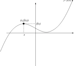
1.2. Graphing Functions. We can make a graph of a function y =f(x) by plotting the points (x, f(x)) in thexy-plane.
y=f(x)
(x,f(x))
x f(x)
Figure 1. Here is how we graph a function y = f(x). We graph the points (x, f(x)).
1.3. Graphing tricks. If we know how to graph a function y =f(x), then we can build up a repertoire of functions by figuring out how this graph changes when we add constants to our equation: f(x) → f(x+c), f(x) → f(c·x), f(x) → c·f(x), or f(x) → f(x) +c. The graph changes by stretching and shifting, depending on the location of the constant. This allows us to have a whole family of functions whose graphs we can draw, by having a few simple examples of functions in mind.
1.4. Examples of Functions. The first examples are lines. To graph a line, we merely have to plot two points, and connect them with a straight line. The first example we have is the line y =x. A general line is of the formy =mx+b. The first constant m is called the slope and the second constant b is called the y-intercept.
The next examples are polynomials. These are functions of the form y = anxn +
an−1x
n−1+· · ·+a
1x+a0, wherean 6= 0. We say that the polynomialy=anxn+an−1x
n−1+ · · ·+a1x+a0 has degree n. A line is a polynomial of degree less than or equal to 1. 1.5. Exponentials and logarithms. Let a be some real number greater than 0. Then we can look at the exponential function y=ax and the logarithmic function y= log
ax.
1.6. Trigonometric functions. There is a family of trigonometric functions, y= sin(x), y = cos(x), y = tan(x), y = csc(x), y = sec(x), and y = cot(x). These are defined for angles x, measured in radians. These functions and their properties will be discussed in recitation.
Lecture 2: Limits and continuity. Slopes and derivatives.
This is the beginning of calculus in earnest. Single variable calculus addresses two major problems.
1. Differential calculus addresses the question, what is the slope of the tangent line to y=f(x) at the point P = (x0, f(x0))?
2. Integral calculus, on the other hand, addresses the question, what is the area under the graph y=f(x) between x=a and x=b?
This week, we will look at the first of these questions, and we will apply the answer to many real-world situations.
2.1. Limits. Suppose we have a function y = f(x) defined on an interval around x = a, but not necessarily at x = a itself. Suppose there is a real number L ∈ R such that as x approaches a (from both the left and the right), f(x) approaches L. In this case, we say,
lim
x→af(x) =L orf(x)→L as x→a.
If no such number exists, then we say there is no limit. We will compute several examples. 2.2. Continuity. We say that a function y=f(x) is continuous at x=a if
1. f(a) is defined; 2. limx→a exists; and
3. limx→a =f(a).
2.3. Slope and derivatives. The goal is to compute the slope of the tangent line to a point (x, f(x)). We do this by computing the slope of secant lines, and taking the limit as the secant lines approach the tangent lines. Thus, the derivative is
df
We will look at several examples of computing derivatives by this definition.
2.4. Velocity and Rates of Change. In recitation, we will see how derivatives appear in the real world as the velocity of a position function, and as a rate of change. We will look at several problems of this nature.
Lecture 3: Differentiation methods.
In this lecture, we will see several methods for computing derivatives, so that we do not always have to use the definition of derivative in order to do computations.
3.1. Rules for differentiation. Here is a list of differentiation rules. We will prove some of these in class, and use them to compute some difficult derivatives.
1. d
3.2. Graphing functions. Derivatives can be used to graph functions. The first derivative tells us whether a function is increasing or decreasing. The second derivative tells us about the concavity of the function. This will be discussed in recitation.
Lecture 4: Max-min problems. Taylor series. Today, we will be using derivatives to solve some real-world problems.
4.1. Max-min problems. The idea with max-min problems is that a functionf(x) defined on an interval [a, b] will take a maximum or minimum value in one of three places:
1. where f′(x) = 0, 2. ata, or
3. atb.
Thus, if we are given a problem such as the following, we know where to look for maximums, minima, the biggest, the smallest, the most, the least, etc.
Example. Suppose we have 100 yards of fencing, and we want to enclose a rectangular garden with maximum area. What is the largest area we can enclose? ♦
We will discuss methods for solving problems like the following.
4.2. Approximations. We can also use the derivative to compute values of functions. Suppose we want to compute√4.02. Then we can take a linear approximation, the tangent line, of √x at x= 4, and compute the approximate value of √4.02 using the tangent line. Linear and quadratic approximations will be discussed.
4.3. Newton’s method. Often times, we would like to know when a function takes the value 0. Sometimes, the answer to this question is obvious, and other times it is more difficult. If we know that f(x) has a zero between x = 1 and x = 2, then we can use Newton’s method to determine the exact value of x for which f(x) = 0. This will be discussed in recitation.
Lecture 5: Taylor Series. Antiderivatives.
In this lecture, we will tie up loose ends of differential calculus, and begin integral calculus.
5.2. Antiderivatives. If we are given a function f(x), we say that another function F(x). is an antiderivativeof f(x) if F′(x) =f(x). We will write
Z
f(x)dx =F(x).
Notice that a constant can always be added toF(x), since d
dxc= 0! We will compute several
anti-derivaties.
Taking antiderivatives can be quite difficult. There is no genearal product rule or chain rule, for example. We have some new rules, however.
5.3. Change of variables. The change of variables formula is the antidifferentiation ver-sion of the chain rule. It can be stated as follows.
Z
f(g(x))g′(x) dx=
Z
f(u) du.
There is also an antidifferentiation version of the product rule. We will discuss this at a later time.
Lecture 6: Area under a curve. Fundamental Theorem of Calculus. I claimed at the beginning of the course that integral calculus attempted to answer a ques-tion involoving the area under a curve. We will see how this is related to antidifferentiaques-tion today.
6.1. Riemann sums. We can approximate the area between a function and the x-axis using Riemann sums. The idea is that we use rectangles to estimate the area under the curve. We sum up the area of the rectangles, and take the limit as the rectangles get more and more narrow. This leads us to the left-hand and right-hand Riemann sums. The left-hand Riemann sum is
Z b
a
f(x)dx= lim ∆x→0
n−1
X
k=0
f(xk)·∆x.
The right-hand Riemann sum is
Z b
a
f(x)dx= lim ∆x→0
n
X
k=1
f(xk)·∆x.
These both converge to the area we are looking for, so long asf(x) is a continuous function. We will make several computations using Riemann sums, and we will look at a few more examples of Riemann sums.
6.2. The Fundamental Theorem of Calculus. We will prove the following theorem. Theorem 6.2.1. If f(x) is a continuous function, and F(x) is an antiderivative of f(x), then
Z b
a
f(x) dx=F(b)−F(a).
We will discuss the implications of this theorem, and look at several examples. Furthermore, we will discuss geometric versus algebraic area.
Lecture 7: Second Fundamental Theorem of Calculus. Integration by parts. The area between two curves.
7.1. Discontinuities and Integration. First, let’s talk about one horrific example where everything seems to go wrong. This will be an example of why we need a function f(x) to be continuous in order to integrate. Consider the function
f(x) =
0 x is a rational number, 1 x is an irrational number.
We can’t graph this function. The problem is, between every two rational points, there is an irrational point, and between every two irrational points, there is a rational point. It turns out that this function is also impossible to integrate. We will discuss why.
7.2. The Second Fundamental Theorem of Calculus. When we were taking deriva-tives, we never really came across functions we couldn’t differentiate. From our little bit of experience with taking indefinite integrals (the ones of the form R
f(x) dx), it doesn’t seem obvious that we can always integrate a function. The Second Fundamental Theorem of Calculus tells us that an integral, or antiderivative, always does exist, and we can write one down.
Theorem 7.2.1. (Second FTC) If f(x) is a continuous function, anda is some real num-ber, then
d dx
Z x
a
f(t) dt=f(x).
This is a by-product of the proof we gave yesterday of the First Fundamental Theorem of Calculus.
7.3. Integration by Parts. I talked about forming the “inverse” of the Product Rule from differentiation to make a rule about taking integrals. This is known asintegration by parts, and the rule is
Z
u dv =u·v−
Z
v du.
f(x)
a b
g(x)
Figure 2. We’re trying to compute the shaded area betweenf(x) and g(x) fromx=ato x=b.
7.4. The area between two curves. Finding the area between two curves looks pretty difficult. Suppose f(x) > g(x). See the figure. If we think about it, though, this is not a hard problem at all! When we think about it, all we have to do is take the area under f(x) on [a, b], and subtract from that the area underg(x) on [a, b]. Thus, the area betweenf(x) and g(x) on [a, b] is
Z b
a
f(x)dx−
Z b
a
g(x) dx=
Z b
a
(f(x)−g(x))dx.
We will discuss some subtleties with this rule.
Lecture 8: Volumes of solids of rotation. Integration techniques. 8.1. Volumes of solids of rotation. Today, we’ll talk about two methods to compute the volumes of rotational solids, volumes by discs and volumes by cylindrical shells.
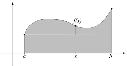
Let us consider for a moment the intuitive idea behind a definite integral. The definite
f(x)
a x b
integral Rb
a f(x)dx is supposed to be an infinitesimal sum (denoted by
Rb
a) along the
x-axis (denoted by dx) of slices with height f(x). The methods we will present to compute volumes of rotation will have a similar intuitive idea.
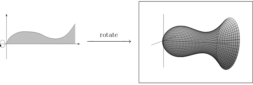
rotate
−−−−−−−→
The goal is to compute the volume of this solid. We have seen some examples of this already in recitation. The first method we will use to compute a volume like this is area by
x A(x)
Figure 3. This shows the slice at the point x. We say that this slice has area A(x).
slices. The volume is the same as infinitesimally adding up the area A(x) of the slices, as shown in the above figure. So
Volume =
Z b
a
A(x)dx .
But this slice is just a circle with radius f(x), so A(x) = π·r2 = π·f(x)2.
Volume =
Z b
a
πf(x)2dx .
function rotated around the y-axis rather than the x-axis. We can think of the volume as the infinitesimal sum of the surface area of the cylinders:
r
h Surface Area = 2πrh
Thus, when computing the volume by cylindrical shells, we have
Volume =
Z b
a
2πxf(x)dx .
Care is required to figure out what the appropriate height function is, and what bounds of integration to use. Furthermore, it is often useful to find a voume such as one of these by integrating with respect to y rather than x. We will see several examples of the cases to which these slices and cylindrical shells apply.
8.2. Integration using partial fractions. A rational function is the quotient of two polynomials, PQ((xx)). It is proper if
deg(P(x)) < deg(Q(x)) and improper if
deg(P(x)) ≥ deg(Q(x)).
An improper rational function can always be reduced to a polynomial plus a proper rational function. For example,
x4 x4−1 =
(x4−1) + 1
x4−1 = 1 + 1
x4−1, and x5
x4−1 =
(x5−x) +x
x4−1 =x+ x x4−1. Furthermore, we can “simplify” or combine terms:
2 x+ 3 +
6 x−2 =
2(x−2) + 6(x+ 3) (x−2)(x+ 3) =
8x+ 14 x2+x−6.
How can we go backwards? This is most easily illustrated with an example. If we start with
2x−11 (x+ 2)(x−3) =
A x+ 2 +
B x−3, how do we find A and B? We know that A and B must satisfy
so
A+B = 2, −3A+ 2B = −11.
We can solve this system, or we can substitute x= 3,−2 in A(x−3) +B(x+ 2) to get A(3−3) +B(3 + 2) = 2·3−11
5B = −5 B = −1, and
A(−2−3) +B(−2 + 2) = 2(−2)−11 −5A = −15
A = 3. So
2x−11 (x+ 2)(x−3) =
3 x+ 2 −
1 x−3. What is this good for? Suppose we want to integrate
Z
2x−11
(x+ 2)(x−3)dx .
We might try to substituteu=x2+x−6, but we would soon see that (2x−11)dx isnot du. So instead, we can split this up:
Z
2x−11
(x+ 2)(x−3)dx =
Z
3
x+ 2dx −
Z
1 x−3dx u = x+ 2
du = dx
w = x−3 dw = dx =
Z 3
udu−
Z 1
wdw
= 3 ln|x+ 2| −ln|x−3|+c
= ln
|x+ 2|3 |x−3|
+c .
A couple of cautionary notes about partial fractions:
1. If there is a term (x−a)m in the denominator, we will get a sum of the form
A1 x−a +
A2
(x−a)2 +· · ·+ Am
(x−a)m ,
where the Ai are all constants.
2. If there is a quadratic factor ax2+bx+cin the denominator, it gives a term Ax+b
8.3. Differential Equations. Finally, if there is time, we will talk a bit about differential equations. A differential equation is an equation that relates a function and its derivatives. For example, consider
dy dx =xy.
The goal is to determine what y is as a function of x. If we treat the term dydx as a fraction, we can separate the variables and put all terms with y and dy on the left-hand side, and all terms with x and dx on the right-hand side. Upon separating, we get
dy
y =x dx. We can now integrate each side to get
ln|y|=
Z dy
y =
Z
x dx= x 2
2 +c. Thus, by raising each side to the power of e, we get
y=C·ex2,
where C is a constant. Differential equations that can be solved in this manner are called differential equations with variables separable. There are many other differential equations which can not be solved in this way. Many courses in mathematics are devoted to solving different kinds of differential equations. We will not spend any more time on them in this course.
Lecture 9: Trigonometric substitution. Multivariable functions. 9.1. Trigonometric substitutions. Today, we’ll discuss trigonometric substitutions a little further. To use the method of trigonometric substitution, we will make use of the following identities.
1−sin2θ = cos2θ , 1 + cot2θ = csc2θ , sec2θ−1 = tan2θ .
If we see an integral with the function √a2−x2 in the integrand, with a a constant, we can make the substitution x=asinθ. Then we have
√
a2−x2 =pa2−a2sin2θ=√a2cos2θ =acosθ.
9.2. Cavalieri’s Principle. Next, we’ll discuss Cavalieri’s Principle. This relates to the disc method we discussed yesterday, although Cavalieri, a contemporary of Galileo, stated the result centuries before the advent of calculus. We will see that this principle is true using calculus.
Theorem 9.2.1. If two solids Aand B have the same height, and if cross-sections parallel to their bases have the same corresponding areas, then A and B have the same volume.
This is clearly true, if we take the volumes by discs. Since the areas of the discs are the same, the volume that we compte when we integrate will be the same.
9.3. Multivariable Functions. Finally, there will be a brief introduction to multivariable functions. We will discuss graphing multivariable functions and multiple integrals, as time permits.
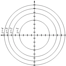
Given a multivariable function z = f(x, y), we can graphs its level curves. These are the curves that we obtain by setting z = a, for constants a. As a varies, we get all of the level curves of the function, which we graph in the xy-plane. For example, we can draw the level curves of the function z =x2 +y2. These will just be circles a =x2 +y2. Using
z=4 z=3 z=2 z=1
Figure 4. This shows the level curves of the func-tion z=x2+y2.
the level curves, we can get a three dimensional view of the function. Now instead of a
Figure 5. This shows the three dimensional graph of the function z =x2+y2. This graph is known as a paraboloid.
make exactly the same Riemann sums as before, but this time instead of just dx, we have dA=dx dy=dy dx.
Lecture 10: Linear algebra
Today, we make a total break from calculus and start linear algebra. We (probably) won’t take another derivative or integral this month! In linear algebra, we will discuss a special class of functions, linear functions
f :Rn→Rm.
We will begin by discussing vectors, properties of vectors, and matrices. 10.1. Vectors. We have vectors inRn. For example,
In general, we will think of vectors in Rnas column vectors, but we may write them as row
vectors in order to save space. We will use v and w to represent vectors. We add vectors component-wise. That is,
We can multiply a vector by a real number a∈R, a scalar, and we do this component-wise as well. We cannot multiply two vectors, but we can take their dot product.
angle θ between them can be computed by
cosθ = v·w ||v|| · ||w||.
This is known as the Law of Cosines. Notice that if the vectors are perpindicular, then the cosine is 0, so the dot product of the vectors must be 0. We also have the Schwartz Inequality, which says
10.2. Matrices. A matrix is anm×n array. Anm×n matrix hasmrows andn columns. We will use a matrix to store data. The (i, j) entry of a matrix is the entry in the ith rown and jth column. Consider the matrix
342 216 47 312 287 29
.
The first row might represent sales in August 2000, and the second sales in August 1999. The first column might reperesent gallons of milk, the second loaves of bread, and the third heads of lettuce. So long as we remember what each row and column represents, we only need keep track of the entries in each position.
As there were vector operations, we also have matrix operations. We can add two ma-trices, so long as they are the same size. As before, addition is entry-wise. For example,
We can also multiply a matrix by a scalar. Again, this is entry-wise. Finally, we can multiply two matrices together, so long as they have the right sizes. We can multiply an m×n matrix by an n×pmatrix to get am×p matrix. The way this happens is if we are multiplying A·B to getC, then the (i, j) entry ofC is the dot product of theith row ofA with thejth column ofB. Notice that the dimension restrictions onA andB are such that these two vectors are the same size, so their dot product is well-defined. For example,
We can also use a matrix to represent the coefficients of linear equations. For example, if we have the system of equations
342x + 216y + 47z = 1041 312x + 287y + 29z = 998 ,
we can find values of x, y and z such that both equations are true. If we let x= 2, y = 1 and z = 3, the equations are true. We will use matrices to find all possible solutions of these equations. We can let a matrix hold the coefficients of these equations. We can write down this system of equations using the matrix eqation
vector of variables, andb is the desired solution vector.
11.1. Gaussian Elimination. First, we will learn an algorithm for solving a system of linear equations. This Gaussian elimination will come up later in the algorithms course, when you have to figure out its time complexity. Suppose you have the following system of equations.
x + 2y − z = 2 x + y + z = 3 .
Subtracting the first equation from the second gives a new system with the same solutions.
x + 2y − z = 2 −y + 2z = 1 .
This system has infinitely many solutions. We can let the variable z take any value, and then x and y are determined. The existence of infinitely many solutions can also occur in the case of three equations in three unknowns. If a coefficient matrixA isn×n, orsquare, then we say that it is singular if A·x=b has infinitely many solutions or no solutions.
Before we give the algorithm for Gaussian elimination, we will define the elementary row operations for a matrix. An elementary row operation on an m×n matrix A is one of the following.
1. Swapping two rows.
2. Multiplying a row by a constant c∈R.
3. Adding ctimes row i of A tod times row j of A. Now, given a system of equations such as
x + 2y − z = 2 x + y + z = 3 , the augmented matrix associated to this system is
1 2 −1 2 1 1 1 3
.
In general, for a system A·x =b, the augmented matrix is
A b
. We say that a matrix is in row echelon form when it satisfies the following conditions.
1. All rows consisting entirely of zeroes, if there are any, are the bottom rows of the matrix.
2. If rows i and i+ 1 are successive rows that do not consist entirely of zeroes, the the leading non-zero entry in rowi+ 1 is to the rightof the leading non-zero entry in row i.
11.2. Inverse matrices. Finally, we will compute the inverse of a matrix. Given asquare matrix A, its inverse is a matrix A−1 such that
A·A−1 =A−1
·A=I,
where I is the identity matrix. To compute the inverse, we take the augmented matrix
A I
, and perform elementary row operations on it until it is in the form
I B
. Then the matrix B is the inverse of A. We will talk about how to prove this in class.
A square matrix is not always invertible. It turns out that a matrix is not invertible if and only if it is singular.
Lecture 12: Matrices. Factorization A =L·U. Determinants.
12.1. Facts about matrices. Here are some interesting facts about matrices, their mul-tiplication, addition, and inverses. Each of the following is true when the dimensions of the matrices are such that the appropriate multiplications and additions make sense.
1. It is notalways true that AB =BA!
2. There is an associative law, A(BC) = (AB)C.
3. There is also a distributive law A(B+C) =AB+AC. 4. (AB)−1 =B−1A−1.
There are also some important types of matrices. We say that an entry of a matrix is on the diagonal if it is the (i, i) entry for some i. A matrix is a diagonal matrix if all of its non-diagonal entries are zero. For example, the matrix
d1 0 0 . . . 0 0 d2 0 . . . 0 0 0 . .. . . . 0 0 0 0 . . . dn
is a diagonal matrix. Diagonal matrices have some nice properties. They commute with each other (that is, CD =DC), and they are easy to multiply. The identity matrix I is a special diagonal matrix: all its diagonal entries are 1. Another type of matrix is an upper triangular matrix. This is a matrix which has zeroes in every entry below and to the left of the diagonal. A lower triangular matrix. is a matrix which has zeroes in every entry above and to the right of the diagonal. Finally, the transpose of an m×n matrix A is an n×m matrix AT, where the rows and columns are interchanged. In this operation, the (i, j)-entry becomes the (j, i)-entry. If a matrix has A =AT, then we say A is symmetric. Notice that (AT)T =A, and that (AB)T =BTAT.
12.2. Factorization of A. We will discuss the factorization A=L·U
be of the form P ·A = L·U. We will discuss how to find L and P if necessary in class. Finally, in the case that A is a symmetric matrix, the factorization A=L·U becomes
A =L·D·LT,
whereDis a diagonal matrix, andLis lower triangular (and henceLT is upper triangular). Our ultimate goal is to factor a matrixA into the form
A=C·D·C−1,
where C is an invertible matrix, and D is a diagonal matrix. This factorization will allow us to compute powers ofA easily, since
An= (C·D·C−1)n =C
·Dn·C−1.
12.3. Determinants. As the name suggests, the determinant of a matrix will determine something about the matrix: if det(A) = 0, then A is a singular matrix. If A is a 2×2 matrix, then
A=
a b c d
,
and det(A) =ad−bc. We will define the determinant for a larger square matrix recursively. Some important properties of the determinant are the following.
1. det(I) = 1 for I the identity matrix.
2. If two rows ofA are the same, the det(A) = 0. 3. If a row of A is all zeroes, then det(A) = 0.
4. If D is a diagonal matrix, then det(D) is the product of the diagonal entries.
5. If A is upper or lower triangular, then det(A) is the product of the diagonal entries. 6. det(AB) = det(A) det(B).
Lecture 13: Vector spaces.
13.1. Application of factorization. We have seen three algorithms thus far. They can be described as follows.
1. Gaussian elimination.
(a) Ax=b gives an augmented matrix
A b
. (b) Use row operations to transform
A b
into
U c
, where U is an upper triangular matrix.
(c) Back solve to find solution(s) x. 2. Gauss-Jordan elimination.
(a) Ax=b gives an augmented matrix
A b
. (b) Use row operations to transform
A b
into
I d
. (c) Read off answer(s) x=d.
3. A=L·U factorization.
(a) Ax=b. Just consider A for a minute. (b) Factor A=L·U.
(c) Ax=L·U(x) =b.
We will discuss each of these algorithms, and see why the last algorithm is the fastest. 13.2. Abstract vector spaces. We are not going to take a step towards the more abstract side of linear algebra. We are going to define a vector space, something like Rn. A vector
space (over R) is a set V along with two operations, + addition of vectors and · scalar multiplication, such that for all vectors v, w, z ∈V and scalars c, d∈R,
1. v+w∈V and v+w=w+v. 2. (v+w) +z =v+ (w+z).
3. There is a zero-vector 0 such that 0 +v =v.
4. For every v, there is an additive inverse −v such that v+ (−v) = 0. 5. c·v ∈V and c·(d·v) = (c·d)·v.
6. c·(v+w) = c·v+c·w. 7. (c+d)·v =c·v+c·w.
Of these, the most important ones are numbers 1 and 5. Most of the other properties are implied by these two. The most important thing to check is that for any two vectors v, w∈V, any linear combinationc·v+d·w of them is also in V.
In class, we will see many examples of vector spaces. We will continue our discussion of vector spaces by defining subspaces. A subset W ⊆ V of a vector space V is a vector subspace if it is also a vector space in its own right. A map L : V1 → V2 is a linear transformation if L(c·v +d·w) =c·L(v) +d·L(w). The kernel or nullspace of a linear transformation is the subset W1 ⊆ V1 such that L(w) = 0 for all w ∈ W1. We write the kernel as ker(L) or N(L). The nullspace of a vector space is a subspace.
Lecture 14: Solving a system of linear equations.
14.1. More vector spaces. First, we will go over several examples of vector spaces. The most important are the row space and column space of a matrix. Given a matrix A, the row space R(A) is the vector space consisting of all linear combinations of the row vectors of A. The column space C(A) is the vector space consisting of all linear combinations of column vectos of A.
14.2. Solving systems of linear equations. We will discuss the complete solution to a systme of linear equations,
A·x=b.
To find the complete solution, we must put the matrix into reduced row echelon form. A matrix is in reduced row echelon form if it satisfies the following conditions.
1. All rows consisting entirely of zeroes, if there are any, are the bottom rows of the matrix.
2. If rowsiandi+ 1 are successive rows that do not consist entirely of zeroes, the leading non-zero entry in row i+ 1 is to the rightof the leading non-zero entry in row i. 3. If rowi does not consist entirely of zeroes, then its leading non-zero entry is 1. 4. If a column has a leading non-zero entry (a 1!) in it in some row, then every other
entry in that column is zero.
arepivot rows. Therank of a matrixAis the number of pivot columns (or rows) that it has when it is transformed into reduced row echelon form. We write rank(A) = r. The pivot variablesare the variables that correspond to the pivot columns. Thefree variablesare the variables corresponding to the free columns.
To find a particluar solution xp to Ax = b, we put
A b
into reduced row echelon form. Then we set the free variables equal to zero, and read off the values of the pivot variables. This is one solution. If a system has free variables, then it has infinitely many solutions. Every solution is of the form xp +xn, where xn is a vector in the nullspace of A, that is Axn = 0. It turns out that we can write down a general solution using the free
variables. We will discuss this precisely in class.
14.3. The fundamental subspaces. We will discuss the four subspaces associatied to an m×n matrix A. The four subspaces are the row space R(A), the column spaceC(A), the nullspace N(A), and the left nullspace N(AT).
Lecture 15: Linear independence. Bases.
15.1. Independence and dependence. Spanning sets. LetV be a vector space. Sup-pose v1,· · · , vn ∈V is some finite set of distinct non-zero vectors. A linear combinationof
these is a sum
c1v1+c2v2 +· · ·+cnvn,
where the ci are real numbers. We say that the set of vectors {v1,· · ·, vn} is linearly
independent if no non-zero comibination of the vectors is zero. That is, if c1v1+c2v2+· · ·+cnvn = 0
for real numbers ci, then all the ci must be zero if the vi are independent.
We say that the set of vectors {v1,· · ·, vn}islinearly dependentif there issome non-zero
linear combination of them that is zero. This means that one of the vectors is a linear combination of some of the other vectors in the subset. That vector depends on the other vectors.
The rank of a matrix can be viewed using the idea of independence. The rank is the number of linearly independent rows (or columns) of a matrix.
We say that a subset of vectors {v1,· · · , vn} in V spans V if every vector v ∈ V is a linear combination of these vectors. We will also call this subset a spanning set.
15.2. Bases and dimension. A basis is a set of vectors {v1,· · · , vn} in V that is both
linearly independent and is a spanning set.
Theorem 15.2.1. If {v1,· · · , vn} and {w1,· · ·, wm} are both bases for a vector space V,
then n =m.
We will prove this theorem in class. This allows us to define dimension. The dimension of a vector space V is the number of vetors in a basis. It turns out that the dimension of the vector space Rn is n, so this definition of dimension conincides with the notion we
already have. We will prove this in class.
1. The row space R(A)⊆Rn has dimension r.
2. The column space C(A)⊆Rm has dimension r.
3. The nullspace N(A)⊆Rn has dimension n−r.
4. The left nullspace N(AT)⊆Rm has dimension m−r.
Lecture 16: Orthogonality and orthonormality. Gram-Schmidt algorithm.
16.1. Orthogonality. We say that a pair of vectors v and w in Rn is orthogonal or
per-pindicular if their dot product is zero, v·w= 0. In vector spaces that are notRn, we must
define what we mean by dot product before we can define orthogonal. Thus, we will restrict our attention to V +Rn.
A basisB ={v1, . . . , vn}ofRnis anorthogonal basisif every pair of vectors is orthogonal.
That is,vi·vj = 0 whenever i6=j. For example, the standard basis of R2 is the basis
B =
1 0
,
0 1
.
This is an orthogonal basis.
Finally, two subspacesW1 andW2 insideV areorthogonal subspacesif for every w1 ∈W1 and w2 ∈ W2, w1 and w2 are orthogonal. Suppose that A is an m×n matrix with rank r. Then the row space R(A) and the nullspace N(A) are orthogonal subspaces of Rm, and the column space C(A) and the left nullspace N(AT are orthogonal subspaces ofRn.
16.2. Orthonormality. We say that a basis B = {q1, . . . , qn} of Rn is an orthonormal
basis if every pair of vectors is orthogonal, and if each vector has length 1. That is,
qi·qj =
0 i6=j 1 i=j .
The standard basis for R2 described above is in fact an orthonormal basis. Orthonormal bases are particularly easy to work with because of the following theorem.
Theorem 16.2.1. If B = {q1, . . . , qn} is an orthonormal basis of Rn and v ∈ Rn is any
vector, then
v =c1q1+· · ·+cnqn,
where ci =v·qi is the dot product of v and qi for all i.
We say that a matrix is an orthogonal matrix if its columns form an orthonormal basis of the column space of the matrix. We will be particularly interested in square orthogonal matrices. The name orthogonal is a bit of a misnomer. Unfortunately, the name has mathematical roots, and so although we would like to call this an orthonormal matrix, we will not. Suppose
Q=
⊤ ⊤ ⊤
q1 q2 · · · qn
⊥ ⊥ ⊥
16.3. Gram-Schmidt algorithm. Suppose B = {v1, . . . , vn} is any basis of Rn. We
Next, the second vector w2 should be perpindicular to w1. We define it to be w2 =v2− v2·w1
w1·w1 w1.
We continue in this manner, and let wi =vi −
for all k. To turn this into an orthonormal bases, we normalize, and set qi =
16.4. Change of basis matrices. Let B be the standard basis of Rn. That is, B =
{e1, . . . , en}, where ei is the vector that has a 1 in the ith position, and zeroes elsewhere.
Let ˜B ={v1, . . . , vn}and ˆB ={w1, . . . , wn}be two other bases of Rn. We will now discuss
the change of basis matrices. Suppose we have a vector
v =
Then we can write this vector as
We may want to write our vector in terms of ˜B. To do this, we need to find constants b1, . . . , bn such that
Solving this equation, we get that
Thus, we say that the change of basis fromB to ˜B is
MB→B˜ =
⊤ ⊤
v1 · · · vn
⊥ ⊥
−1
.
The change of basis matrix from ˜B toB is
MB˜→B =
⊤ ⊤
v1 · · · vn
⊥ ⊥
.
Finally, if we want to change basis from ˜B to ˆB, then the change of basis matrix is MB˜→Bˆ =MB→Bˆ ·MB˜→B.
We seem to have multiplied in the wrong order. We will discuss this in class, and compute several examples.
Lecture 17: Eigenvalues, eigenvectors and diagonalization.
17.1. Eigenvalues and eigenvectors. For a matrixA, the eigenvalues of A are the real numbers λ such that
A·v =λ·v for some vector v. Let’s explore this equation further.
A·v = λ·v = (λ·I)·v Av−λIv = 0
(A−λI)·v = 0 This last line will have a nonzero solution v if and only if
det(A−λI) = 0.
Thus, we find the eigenvalues of A by finding roots of the polynomial det(A−λI) = 0.
An eigenvector of a matrixA is a vector v such that A·v =λ·v,
for some real number λ. Once we know what the eigenvalues are, we can find associated eigenvectors.
17.2. Diagonalization. IfAis a matrix, and there is a diagonal matrixDand an invertible matrix P such that
A=P ·D·P−1, then we say that A is diagonalizable.
Theorem 17.2.1. A matrix A is diagonalizable if it has n distinct eigenvalues. In this case, if λ1, . . . , λn are the eigenvalues and v1,· · · , vn are the eigenvectors, then
In the case when the eigenvalues are not distinct, the matrix may or may not be diago-nalizable. In this case, there is still a canonical form known as the Jordan canonical form. We will discuss this in class. Some matrices may be diagonalizable over R, but they are over C. We will see an application of diagonalization tomorrow.
Lecture 18: Fibonacci numbers. Markov matrices.
18.1. Fibonacci numbers. In the year 1202, the Italian mathematician Fibonacci pub-lished a book in which he defined a certain sequence of numbers. The so-called Fibonacci numbers are defined by the relation
Fn=Fn−1+Fn−2, and F0 = 1 andF1 = 1. This sequence is
0,1,1,2,3,5,8,13,21,34,55, . . . .
We can use diagonalization to write a closed form equation for thenth Fibonacci number. If we put two values in a vector,
So if we could easily compute
1 1 1 0
n
,
we could easily compute thenth Fibonacci number. If we diagonalize the matrix
1 1 1 0
then we can easily compute its nth power. We will do this in class, and come up with the formula
Fn =
1 √ 5
1 +√5 2
!n+1
− 1− √
5 2
!n+1
.