Modeling insulin kinetics: responses to a single oral glucose
administration or ambulatory-fed conditions
Yongwimon Lenbury *, Sitipong Ruktamatakul, Somkid Amornsamarnkul
Department of Mathematics,Faculty of Science,Mahidol Uni6ersity,Rama6Rd.,Bangkok10400,Thailand
Received 24 August 2000; accepted 28 August 2000
Abstract
This paper presents a nonlinear mathematical model of the glucose – insulin feedback system, which has been extended to incorporate theb-cells’ function on maintaining and regulating plasma insulin level in man. Initially, a gastrointestinal absorption term for glucose is utilized to effect the glucose absorption by the intestine and the subsequent release of glucose into the bloodstream, taking place at a given initial rate and falling off exponentially with time. An analysis of the model is carried out by the singular perturbation technique in order to derive boundary conditions on the system parameters which identify, in particular, the existence of limit cycles in our model system consistent with the oscillatory patterns often observed in clinical data. We then utilize a sinusoidal term to incorporate the temporal absorption of glucose in order to study the responses in the patients under ambulatory-fed conditions. A numerical investigation is carried out in this case to construct a bifurcation diagram to identify the ranges of parametric values for which chaotic behavior can be expected, leading to interesting biological interpretations. © 2001 Elsevier Science Ireland Ltd. All rights reserved.
Keywords:Insulin kinetics; Mathematical model; Periodicity; Chaotic dynamics
www.elsevier.com/locate/biosystems
1. Introduction
It has been established (Bajaj and Rao, 1987) that the secretion of insulin and its biological effectiveness in response to a glucose load is deter-mined mostly by the number and function of
b-cells in the pancreas, and the peripheral resis-tance to insulin action. Diabetes can arise from insulin deficiency or insulin resistance and several studies have been carried out to determine their
relative contributions toward a patient’s hyper-glycemia (Turner et al., 1979). A number of math-ematical models have been proposed (Ackerman et al., 1964; Geevan et al., 1990) to explain the relationships between the concentrations of cose and insulin in plasma in response to a glu-cose load.
These models are usually too complex to be fitted to the small amount of clinical data avail-able. Moreover, the data is generally of glucose concentrations only and has been collected over a time scale of an experiment, which is too short for the model’s verification (Bajaj and Rao, 1987). * Corresponding author.
E-mail address:[email protected] (Y. Lenbury).
More importantly, most models prove not to be consistent enough with known physiological data. On comparing mathematical models, it is no longer sufficient to match numerical simulations to experimental data and choose the best fitting model. We are in a better position if the model can be shown to admit the same dynamic behav-ior exhibited by real data. Specifically, if sustained oscillatory patterns are observed in the system under study, a model which does not admit such a qualitative behavior must be discarded. As Ack-erman et al. (1964) have observed, body or natu-ral rhythms range from very fast ones, such as those of the electro-encephalogram, to very slow ones, such as seasonal variations. Some of these rhythms are induced by the external environment, while others are characteristic of the living organ-isms. Apart from the oscillations of long periodic-ity such as those of about 24 h, several physiological variables also show shorter rhythms, which are often regarded as a complication that somehow must be avoided or compensated for in the design of experiments in biology and medicine. Instead, these rhythms should be stud-ied and used as qualitative parameters of the biological system. It was proposed by Ackerman et al. (1964) that the analysis of cyclic variations and periodicity in a system could prove to be a useful tool to help distinguish health from disease. A recent model for insulin kinetics, studied by Geevan et al. (1990), involves four variables, in-corporatingb-cell kinetics, a glucose – insulin feed-back system and a gastrointestinal absorption term. Analysis of the model (Bajaj and Rao, 1987) showed that only damped oscillations were admit-ted in response to an instantaneous oral glucose administration. Several studies have, however, re-ported persistent cyclic patterns in the plasma glucose and insulin concentrations in man and monkeys (Turner et al., 1979; Tasaka et al., 1994). In another study by Molnar et al. (1972), where immunoreactive insulin measurements were made from ambulatory-fed subjects, plasma insulin and glucose patterns in diabetics showed chaotic be-havior during the 48-h observation period.
We, therefore, extend the above mentioned model to take into account the role of the number ofb-cells in the regulation of plasma insulin level,
following the results presented by Turner et al. (1979) in which theb-cells function in the negative feedback loop appears to have a predominant role in regulating both the basal plasma glucose and insulin concentrations.
We show, by a singular perturbation analysis, that the model will admit sustained oscillations for certain ranges of the system parameters. Moreover, when a term is incorporated to simu-late the responses to an ambulatory-fed condition, we discover that chaotic behavior can be expected in the system for certain ranges of the system parameters, yielding irregular patterns consistent with the physiological data reported by Molnar et al. (1972).
2. Model development
Here, we derive an extended model by making the following assumptions. If x and y represent the differences in the plasma insulin and glucose concentrations from their respective fasting (basal) concentrations, and z represents the den-sity of the pancreatic b-cells in the proliferative phase, then the rate of change of x satisfies the following rate equation.
dx
dt=R1y−R2x+C1 (1)
where the first term describes the increase in the insulin concentration due to the increase in the plasma glucose concentration; the second term describes the reduction in x due to its access amount, while C1, is the rate of increase in x in the absence of y andx.
Since b-cells function in a negative feedback loop has been established to take a predominant role in regulating both the basal plasma glucose and insulin concentrations (Bajaj and Rao, 1987; Lenbury et al., 1996), it is reasonable to assume that the rates R1, R2 and C1 in Eq. (1) should depend on the density of b-cells in the prolifera-tive phase z. Eq. (1) thus becomes
dx
where linear dependence onzis assumed while r1, r2andclare positive constants. The system is thus considered to be a self-regulative one in a normal subject, where basal plasma glucose level is pre-dominantly determined by insulin secretion from normalb-cells. A decreased number of cells would maintain a normal basal plasma insulin concen-tration by operating at an increased secretory rate per cell. This is reflected by the second term in Eq. (2), which becomes smaller in magnitude as z decreases so thatxwill be reduced at a slower rate in the event that the number of cells becomes smaller.
As for the plasma glucose level y, if there is a decrease in insulin secretion due to a reduction to 1/Nof the normal number,n, ofb-cells, the basal plasma glucose will increase until nearly normal basal insulin levels are obtained (Bajaj and Rao, 1987). Thus, the plasma glucose level is a function of the b-cell capacity, N/n. Therefore, plasma glucose is assumed to satisfy the following rate equation.
dy dt=
R3N
z −R4x+C2+w(t) (3)
where the first term accounts for the hyperbolic increase in ydue to a reduction in the number of
b-cells, supported by the study of Turner et al., (1979) mentioned previously. The second term accounts for the reduction inydue to the regula-tive effect of plasma insulin, whileC2accounts for the change inyin the absence ofxandz. The last term in Eq. (3) corresponds to the variation in the gastrointestinal absorption with time, accounting for the absorption by the intestine and the subse-quent release of glucose into the bloodstream.
Finally, the density of pancreaticb-cells in the proliferative phase satisfies the following equation used in the work of Rao et al. (1990):
dz
dt=R5(y−yˆ)(T−z)+R6z(T−z)−R7z (4)
where yˆ is the difference between the normal glucose level and its basal concentration,T is the total density of dividing and non-dividingb-cells, whileR5, R6, andR7 are rate constants. The first term accounts for the increase in z due to the interaction between the plasma glucose above the
basal level and the non-dividing b-cells, while the second term represents the increase in the dividing
b-cells from the interaction between the dividing and non-dividing cells. The last term is the rate of reduction in the cells density, proportional to its current level with a rate constant R7.
Thus, our reference model consists of Eqs. (2) – (4).
3. Single oral glucose administration
When a single oral glucose administration is utilized, a gastrointestinal absorption term w(t) is assumed to have the form
w(t) 1
p+eat (5)
which means that the absorption by the intestine and the subsequent release of glucose into the bloodstream takes place at an initial rate
w0= 1
p+1 (6)
and then falls off exponentially with time (Rao et al., 1990).
On substituting Eq. (5) into Eq. (3) and differ-entiating w(t), we can eliminate the time depen-dence of the termw(t) by considering instead the following system of four autonomous differential equations
4. Singular perturbation analysis
absorption. Thus, ifais high, the gastrointestinal absorption process equilibrates very quickly to the steady state w=0 of Eq. (10), which is stable. This means that as time passes w becomes infi-nitesimally small and the system model reduces to Eqs. (7) – (9) with w=0.
In order to analyze the resulting model equations (Eqs. (7) – (9)) with w=0 by a singular perturbation technique, we scale the dynamics of the three remaining hierarchical components of the system, namely x, y and z, by means of two small dimensionless positive parametersoand d.
Letting zˆ=T, r3=R3N/o, r4=R4/o, r5= R5/od,r6=R6/od,r7=R7/od, andc2=C2/o, we are led to the following system of differential equa-tions.
which means that during transitions, when the right sides of Eqs. (11) – (13) are finite but differ-ent from zero, y; is of the order o, and z; is of order od. Thus, we have assumed that insulin formation has faster time response than that of plasma glucose, and the b-cells proliferation pos-sesses the slowest dynamics.
It is well known (Muratori, 1991; Muratori and Rinaldi, 1992; Lenbury et al., 1996) that the sys-tem (Eqs. (11) – (13)), whenoandd are small, can be analyzed with the singular perturbation method which, under suitable regularity condi-tions, allows approximation of the solution of the system by a sequence of simple dynamic transi-tions occurring at different speeds. The resulting curve, composed of these transitions, approxi-mates the actual solution in the sense that the real trajectory is contained in a tube around the curve, and that the radius of the tube goes to zero with o, and d.
4.1. On the manifold f=0
This consists of the trivial manifold z=0 and the nontrivial one given by the equation
x=r1 r2
y+c1 r2
(14)
The above equation describes a plane in the (x, y, z)-space which is parallel to the z-axis. It intersects the (x, z)-plane along the line
x=c1 r2
x1 (15)
as shown in Fig. 1.
4.2. On the manifold h=0
This is the surface
y=p(z)yˆ−r6z
Settingp%(z)=0, one obtains
z=zˆ9
'
r7zˆ r6Since it is necessary thatz5zˆ, we consider only the critical point where
z=zˆ−
'
r7zˆfor positive parametric values. Thus, z is a mini-mum at the point z=z1, on this surface. Substi-tuting z1 into Eq. (16), one obtains
p(z1)=yˆ− 1
r5
(r7−r6zˆ)2y1 (20) Also, if z=0 on this surface, then
z=zˆ
which is where the manifold intersects the (x, y)-plane, as shown in Fig. 1.
We observe further that the slow manifold given by Eq. (16) is parallel to the x-axis and intersects the (y,z)-plane along a curve on which y becomes a minimum at the point where z=z1. Moreover, the manifold h=0 intersects the plane of the manifold f=0 along the parabolic curve given by the equation
x=c(y,z)
1 r2
[r1y+c1+r7z−r5(y−yˆ)(zˆ−z)
−r6z(zˆ−z)] (21)
Substituting y1 and z1, in the above equation, we obtain
also shown in Fig. 1.
On the other hand, on substituting y=yˆ and z=0 in Eq. (21), we obtain
x=1 r2
[r1yˆ+c1]x3 (23)
However, on considering Eqs. (22) and (23), we find thatx3\x2for all positive parametric values. Now, for a constant y, c is a decreasing func-tion ofzon the interval (0,z1), that is,xdecreases along the curve given by Eq. (21) from the point (x, y, z)=(x3, yˆ, 0), or point P in Fig. 1, to the point (x,y,z)=(x2,y1,z1), or point D, along the curve PD in Fig. 1.
4.3. On the manifold g=0
This is the cylindrical surface given by
x=f(z)r3 r4z
+c2 r4
(24)
which is parallel to the y-axis and intersects the (x,z)-plane along a hyperbola. As ztends toward infinity along this surface, x tends toward the value c2/r4.
Since f(z) is a monotonically decreasing func-tion of z, ifz1\0 thenxis decreasing forzin the
Thus, by requiring that
zˆ\r7 r6
(28)
then, on considering Eqs. (18) and (20), we are assured that y1\0 and z1\0.
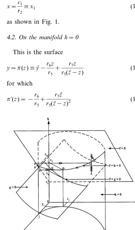
Under these conditions, the shapes and relative positions of the equilibrium manifolds f=0,g= 0, and h=0 will be as depicted in Fig. 1, where three arrows indicate fast transitions, two arrows indicate intermediate ones, while a single arrow indicates slow ones.
Thus, a system initially at a generic point, say point A of Fig. 1, will make a quick transition to the plane given by Eq. (14) on the fast manifold f=0 (point B in Fig. 1), since the signs offassure us that this part of the manifoldf=0 is stable. As the plane wheref=0 is approached,y has slowly become active. A transition at an intermediate speed is made along f=0 in the direction of decreasingy, sincegB0 here, to the point C on a stable part of the curvef=h=0. From the point C, a slow transition is then made along this curve in the direction of decreasing y, since g is still negative here.
Once the point D is reached, the stability of the manifold is lost, a catastrophic transition brings the system to point E on the manifoldz=0 where it intersects the plane given by Eq. (14). Conse-quently, the system will slowly develop along this line in the direction of increasingy, sincegis now positive.
At a point F on the plane z=0, the stability will again be lost and a quick transition will bring the system back to the point G on the stable branch of the curvef=h=0, before repeating the same previously described path, thereby forming a closed cycle GDEFG. Thus, the existence of a limit cycle in the system for o and d sufficiently small is assured. The exact solution trajectory of the system will be contained in a tube about this closed curve, the radius of which tends to zero with o and d.
The above arguments can be summarized by the following theorem.
Theorem 1. If inequalities (Eqs. (26) – (28)) hold, and o and d are sufficiently small, then the system of Eqs. (11) – (13) has a global attractor, in the positi6e octant of the phase space, which is a limit
cycle composed of a concatenation of catastrophic transitions occurring at different speeds.
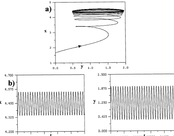
A computer simulation of Eqs. (11) – (13) is presented in Fig. 2a, with parametric values cho-sen to satisfy inequalities (Eqs. (26) – (28)) iden-tified in the above theorem. The solution trajectory, projected onto the (y, x)-plane, is seen here to tend towards a limit cycle as theoretically predicted. The corresponding time series of insulin (x) and glucose (y) are shown in Fig. 2b.
5. Ambulatory-fed conditions and chaotic behavior
We now extend our model to incorporate tem-poral glucose absorption in order to model the responses of a subject under ambulatory-fed con-ditions. The term w(t) in Eq. (3) is then taken in this case to assume the sinusoidal form
w(t)ksinvt (29)
We then remove the explicit dependence on time of the above oscillatory term by letting
u=cosvt
and
6=sinvt
which transforms the model equations into the following five-dimensional system of autonomous differential equations.
Fig. 2. A computer simulation of the model system of Eqs. (11) – (13) with parametric values chosen to satisfy the conditions identified in the text for which periodic solutions exist. The solution trajectory, projected onto the (y,x)-plane, is seen in Fig. 2a to tend toward a stable limit cycle as theoretically predicted. The corresponding time series of plasma insulin (x) and glucose (y) are shown in Fig. 2b. Here, o=0.1; d=0.01; r1=0.2; r2=0.1; r3=0.1; r4=0.1; r5=0.1; r6=0.1; r7=0.05; cl=0.1; c2=0.1;
yˆ=1.24;zˆ=2.0; andN=0.1.
discovered by some researchers (Hastings and Powell, 1991; Lenbury et al., 1999) that one may be able to generate chaos in a nonlinear system which already exhibits limit cycle behavior, we choose parametric values that would lead to cy-cling in thex,yandzcomponents, guided by our work in the previous section.
We then let the system run for 105
time steps, and examining only the last 8×10⁴ time steps to eliminate transient behavior. Using the values ofzˆ between 0.985 and 1.038, and changing zˆin steps of 10−5, the relative maximum values x
max of x
are collected during the last 8×l04 time steps. They are then plotted as a function ofzˆas shown in Fig. 3. We discover in this bifurcation diagram the appearance of a period doubling route to chaos, which resembles the dynamics of one-di-mensional difference equations such as the logistic population model. Thus, the system of Eqs. (30) – (34) appears to exhibit chaotic dynamics for val-ues ofzˆ between 1.000 and 1.038.
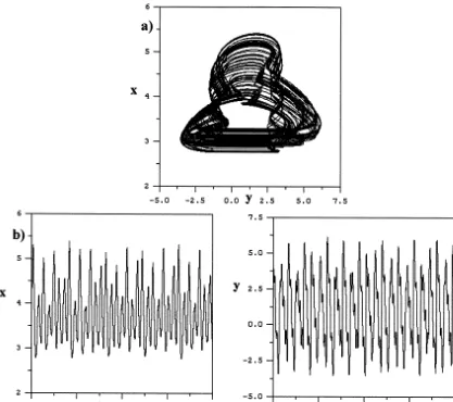
A computer simulation of the model system (Eqs. (30) – (34)), with parametric values chosen under the above mentioned guidelines and zˆ= 1.01 in the chaotic range, is presented in Fig. 4a, showing the strange attractor projected onto the (y, z)-plane, and the corresponding chaotic time courses of plasma insulin (x) and glucose (y) are presented in Fig. 4b.
6. Discussion and conclusion
In a situation where chaotic dynamics are ob-served, a small change in the initial conditions may lead to drastically different dynamic behav-ior. Thus, even a slight perturbation in the insulin concentration may lead to unpredictable results through time.
administration combined with regular eating and exercise schedules is ineffective in maintaining blood glucose within normal limits. Rather, there can be apparently irregular fluctuations (Molnar et al., 1972), for example, in blood glucose moni-tored upon rising. The unpredictability of glucose or insulin patterns could generate many control problems. A low insulin concentration can result in polyuria and circulatory shocks. Conversely, a high insulin concentration indicates possibility of convulsion, sympathetic over-activity and loss of consciousness.
On the other hand, a reduction in blood glucose levels below 45 – 55 mg/100 ml for a continued interval of time will lead to an impairment of brain function, tremors, and convulsions due to activation of the sympathetic nervous system and, ultimately, death (Norman and Litwack, 1997). Hence, it is necessary to develop protocols for insulin administration based on a knowledge of ambient blood-sugar levels and an understanding of the dynamics of the glucose control system.
In the paper by Tasaka et al. (1994), clinical data was reported where irregular patterns were observed in the time courses of plasma insulin levels. Earlier, Molnar et al. reported immunore-active-insulin (IRI) measurements made during studies in ambulatory-fed subjects. It was pointed
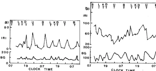
out that in normal subjects, an IRI increase oc-curred after every increased blood glucose (BG). In an unstable diabetics, however, there were fewer IRI increases and these increases bore a less regular relationship in time to the BG increases which followed the meals. We observe that the reported IRI and BG patterns, shown in Fig. 5, appear more irregular in an unstable diabetics than in a normal subject.
We have been able to discover in our model the possibility of chaotic behavior with the appear-ance of a strange attractor for the values of zˆ in the approximate range 1.000BzˆB1.038. On the other hand, periodic oscillations in the three com-ponents of our system are observed if 0.98BzˆB 1.0, and other parametric values are as in the bifurcation diagram shown in Fig. 3. We have thus found that the bifurcation parameter, which delineates various dynamic behaviors in our sys-tem is the total density zˆof b-cells.
In comparison, it was discovered in our earlier study (Lenbury et al., 1996) that the critical parameter which differentiates the various dynam-ical behaviors clindynam-ically observed in the electrdynam-ical activities in the b-cells is, in fact, that which is related to cell shape and volume, among other channel conductance related parameters. It has been well established that such electrical activities
Fig. 3. Bifurcation diagram for the model system of Eqs. (11) – (13) witho=0.1,d=0.01,r1=0.15,r2=0.12,r3=0.05,r4=0.03,
Fig. 4. A computer simulation of the model system of Eqs. (11) – (13) with parametric values of Fig. 3 andzˆ=1.01 in the chaotic range, showing a strange attractor projected onto the (y,z)-plane in Fig. 4a. The corresponding time series of plasma insulin (x) and glucose (y) are shown in Fig. 4b.
are closely related to insulin secretion and the regulation of plasma glucose. Chaotic behavior in the potential difference component, which will result when the critical parameter falls within certain ranges can be indicative of irregularities in the underlying mechanisms of the system under study.
To summarize, we have demonstrated in this paper that our system model consisting of Eqs. (7) – (9) can exhibit sustained oscillations after an initial dose of glucose. It can also exhibit chaotic dynamics under ambulatory-fed conditions,
con-sistent with the reported clinical data. Our investi-gation demonstrates how the frequency of IRI increases is interfered with by the added frequency of meals being fed. When synchrony is disturbed further in a patient with impaired glucose – insulin regulation system, a period doubling route to chaotic dynamics may be observed.
glu-Fig. 5. Variations in IRI (in mg/100 ml) and BG (inmU/ml) during 48 h continuous monitoring. Clocktime is shown in hours and major meals were taken at 6-h intervals. B, breakfast; L, lunch; K, snack; D, dinner; U, supper; normal subjects in (a); diabetics in (b). Data is taken from Molnar et al. (1972).
cose pattern of a normal subject shows very low peaks, while the insulin level oscillates between zero and maximum levels of no more than 80
mU/ml. The diabetic patient’s data in Fig. 5b, on the other hand, shows higher glucose peaks, and the plasma insulin oscillates between 20 and 100
mU/ml. On comparing our simulation results in Fig. 2, for the periodic case, and Fig. 4, for the chaotic case, we see that our model exhibits the same qualitative difference, which has been ob-served clinically in the corresponding cases of normal subjects and diabetic patients.
Thus, this study shows how such insights gained from our analysis can have clinical utility in distinguishing health from disease. More in-depth studies and sufficient amounts of additional data should allow us to establish a stronger link-age between the dynamic behavior of the model and the clinically observed patterns, and lead us in the right direction towards our being eventually in the position to make certain reliable predictions regarding the control strategies and effective ther-apy of diabetes mellitus.
Acknowledgements
The authors would like to extend their deepest appreciation to the Thailand Research Fund for supporting this research project (contract number RTA/02/2542).
References
Ackerman, E., Rosevear, J.W., McGuckin, W.F., 1964. A mathematical model for glucose-tolerance test. Phys. Med. Biol. 9 (2), 203 – 213.
Bajaj, J.S., Rao, G.S., 1987. A mathematical model for insulin kinetics and its application to protein-deficient (malnutri-tion-related) diabetes mellitus (PDDM). J. Theor. Biol. 129, 491 – 503.
Geevan, C.P., Rao, S., Rao, G.S., Bajaj, J.S., 1990. A mathe-matical model for insulin kinetics III. Sensitivity analysis of the model. J. Theor. Biol. 147, 255 – 263.
Hastings, A., Powell, T., 1991. Chaos in a three-species food chain. Ecology 72 (3), 896 – 903.
Lenbury, Y., Kumnungkit, K., Novaprateep, B., 1996. Detec-tion of slow – fast cycles in a model for electrical activity in the pancreaticb-cell. IMA J. Math. Appl. Med. Biol. 13, 1 – 21.
Lenbury, Y., Rattanamongkonkul, S., Tumrasvin, N., Amorn-samarnkul, S., 1999. Predator prey interaction coupled by parasitic infection: limit cycles and chaotic behavior. Math. Comp. Model. 30, 131 – 146.
Molnar, G.D., Taylor, W.F., Langworthy, A.L., 1972. Plasma immunoreactive insulin patterns in insulin-treated diabet-ics: studies during continuous blood glucose monitoring. Mayo Clin. Proc. 47, 709 – 719.
Muratori, S., 1991. An application of the separation principle for detecting slow – fast limit cycles in a three-dimensional system. Appl. Math. Comput. 43, 1 – 18.
Muratori, S., Rinaldi, S., 1992. Low- and high-frequency oscillations in three-dimensional food chain systems. 52, 1688 – 1706.
Norman, A.W., Litwack, G., 1997. Hormones, second ed. Academic Press, California.
Tasaka, Y., Nakaya, F., Matsumoto, H., Omori, Y., 1994. Effect of aminoguanidine on insulin release from pancreatic islet. Endocr. J. 41 (3), 309 – 313.
Turner, R.C., Holman, R.R., Mattthews, D.R., Hockaday,
D.R., Peto, J., 1979. Insulin deficiency and insulin resistance interaction in diabetes: estimation of their relative contribu-tion by feedback analysis from basal plasma insulin and glucose concentrations. Metabolism 28 (11), 1086 – 1096.