ON THE OPTIMAL REPRESENTATION OF VECTOR LOCATION USING
FIXED-WIDTH MULTI-PRECISION QUANTIZERS
K. Sahr
Dept. of Computer Science, Southern Oregon University, Ashland, Oregon, 97520 USA – [email protected]
KEY WORDS: Data Structures, Representation, Precision, Multiresolution, Global, Hierarchical
ABSTRACT:
Current generation geospatial applications primarily rely on location representations that were developed for the manipulation and display of planar maps of portions of the earth’s surface. The next generation of digital earth applications will require fundamentally new technological approaches to location representation. Improvements in the efficiency of the representation of vector location can result in substantial performance increases. We examine the advantages and limitations of the most common current approach: as tuples of fixed-width floating point representations of real numbers, and identify a list of desirable design features for an optimal replacement system. These include the use of explicitly discrete integer indexes, the use of an optimal quantification scheme, and the ability to represent point locations at multiple precisions, including the capability to exactly represent key point locations, and the ability to encode multi-precision quantizations. We describe a class of planar systems that meet these criteria, which we call Central Place Indexing (CPI) systems. We then extend these systems to the sphere to provide a class of optimal known fixed-width geospatial vector location representation systems we call CPI43 systems.
1. INTRODUCTION
A recent convergence of factors, including pervasive GPS-located mobile computing devices, vast readily available quantities of global imagery and geo-referenced data, and consumer-level 3D cloud-based visualization and analysis platforms, has resulted in a rapidly accelerating demand for the computer processing of vast quantities of diverse and often distributed geospatial data — data for which a primary access key is a computer representation of location on the surface of the Earth. The current geospatial computing software infrastructure has been built over the past half-century upon the foundations laid-out by GIS researchers and advanced end users. These communities have defined the core semantics and operations of location abstract data types. These communities have also guided the development of the primary approaches currently used to represent geospatial location, based on location representations that were developed for the manipulation and display of planar maps of portions of the earth’s surface. But the next generation of geospatial applications will include advanced “digital earths” — 3D virtual globes that will allow a broad spectrum of users, including scientists, educators, businesses, and individuals, to interactively visualize, analyze, model, manipulate, and generate geospatial big data (Goodchild, 2010; Goodchild et al., 2012; Yu & Gong, 2012). New approaches to geospatial computing will need to be developed to meet the needs of these next generation applications. Because data structures for the representation of location are so pervasive, even small improvements in efficiency or representational accuracy in these data structures can result in substantial performance increases in an overall system.
Arguably the most fundamental of location types is point or vector location. The traditional geospatial data end-user approach to specifying point locations — both before and since the advent of geospatial computing — have been as a two- or three-tuples of real numbers, most commonly either geographic (latitude/longitude) coordinates, planar Cartesian coordinates in some map projection space, or Earth-Centered, Earth-Fixed
reference frame coordinates. This approach gives users the optimal flexibility to perform arbitrary manipulations of these point locations by applying analytic geometry techniques to potentially exact real numbers.
By far the most common representation of a real number — within geospatial applications as well as across all computing — is as a fixed-width floating point (FWFP) value; that is, using a fixed number of bits, with some of those bits encoding a mantissa and some encoding an exponent. This representation provides the end-user with an approximate surrogate for their familiar real numbers, to which can be applied computer implementations of familiar real number operations. This approach has been enabled and supported by the widespread development and availability of algorithms and hardware (such as floating point processors) designed to optimize the manipulation of vectors of FWFP values. The representation of point locations using tuples of FWFP values has proven sufficient to form the very substrate upon which current geospatial computing, with all its impressive achievements, has been constructed. But as powerful and convenient as this approach has been, certainly it would be difficult to argue that it is the most efficient representation possible for point locations, under most reasonable definitions of the term “efficient”.
quantizations. We describe a class of planar systems that meet these criteria, which we call Central Place Indexing systems. Finally, we extend these systems to the sphere to provide a class of optimal known fixed-width geospatial vector location representation systems.
2. THE LIMITATIONS OF FIXED-WIDTH FLOATING POINT VECTOR LOCATION REPRESENTATIONS FWFP representations will continue to be important to end users for the foreseeable future. But we must distinguish between the values that our program presents to end users — such as decimal numbers, with a specific precision — and the internal representation of those numbers as discrete binary values with some indeterminate precision. The decimal number that the end user sees is not the actual location key value, but is generated from that internal key representation, with the assistance of metadata (such as the number of base 10 significant digits in the value) when it is available. This fact alone means that a FWFP representation will result in representational rounding errors for an infinite number of decimal values. For example, an analyst who wants to work with a latitude value of exactly 7.55° will find that that number has an infinite binary representation, and thus the actual decimal number stored will be 7.54999...°. The FWFP representational conversion processing may be supported by hardware and thus be very efficient; indeed, in general the widespread availability of floating point hardware has traditionally given FWFP representations an immediate efficiency advantage over other potential representations for a wide range of operations. But given the speed and ease with which new processor circuitry now goes from algorithm definition to implementation, even this hardware advantage has ceased to be a real obstacle to introducing new representations. We may encode our point location key value using the most efficient internal representation, and then generate or store other point location representations (such as decimal latitude/longitude) as needed. For efficiency, that conversion can itself be encoded in hardware.
Modern GPS-equipped mobile computing devices exemplify the requirements of advanced real-time geospatial processing in a resource-constrained environment. My Apple iOS device reports to me that I am currently at latitude/longitude coordinates (42.18614334, -122.697120) with an accuracy of +/-10 meters; that is, the reported location lies at the center of a circle with a “radius of uncertainty” (Apple Inc., 2010) of 10 meters. The documention for Android devices (Android Open Source Project, 2013) gives more detail, indicating that a reported accuracy is “the radius of 68% confidence.” In neither system is any information given about the precision or number of significant digits in the latitude/longitude FWFP representation itself. In fact, the very concepts of accuracy and precision have such varied practical definitions that it is difficult to make definitive statements about their meaning in any given technological system. In classical measurement theory accuracy indicates how close a measurement is to the actual location value, while precision indicates how close together the values of repeated measurements of the same position are. But these definitions do not always apply in practice; for example, the ISO 5725 standard (ISO, 2012) defines experimental accuracy as the combination of both “trueness” and “precision”. And when referring to FWFP representations the term precision normally (e.g., IEEE Computer Society, 2008) refers to the number of significant digits that are preserved by the representation. Since the precision applies individually to each component of a 2-tuple FWFP representation, the resulting region of uncertainty is square, rather than circular, as it is in the
standard expression of location accuracy. But from the standpoint of location representation, terms like accuracy, precision, and resolution all refer to the degree to which a particular location address reduces our uncertainty concerning a point location value. An ideal vector location representation would implicitly correspond to a region on the surface of the earth in which the point lies, with the area of that region proportional to the degree of location uncertainty, and applications should be able to identify that region without resorting to meta-data. An ideal representation system would also be capable of providing multiple representations of the same location, each corresponding to a different degree of location uncertainty. To avoid confusion, in the remainder of this paper we will use the term precision to indicate the degree to which a particular location representation reduces the uncertainty associated with that location position.
Any representation of the real numbers on a digital computer is necessarily finite and discrete, while the real numbers themselves are infinite in extension, continuous, and infinitely divisible. Consequently, performing even the most fundamental operations on these representations has the potential to introduce and/or propagate rounding error. For example, two FWFP location representations are usually considered “equal” if the distance between them is less than some relatively small number. This makes it impossible to distinguish between two addresses which represent point locations that are distinct, yet very close, and two addresses which are intended to indicate the same location but which differ due to rounding error. This problem is compounded, when, as described above, the representations do not clearly encode their precision. In geospatial applications the result of a location equality test may well have significant semantic implications; it might, for instance, be an important decision point in determining the application’s future execution path. And while it is often possible to bound the rounding error due to a single calculation or even an entire single application execution, complex geospatial computing applications often involve interactions between multiple programs and data sets, often with location representations with varying precisions. In such situations it can be very difficult, if not impossible, to bound the cumulative round-off error present in the final system results, which may themselves serve as inputs into additional geospatial processing.
degree of geometric regularity. On the plane a hexagonal distribution is the best known for estimating continuous spatial functions using kriging (Olea, 1984), and such a distribution is 13.4% more efficient than a square distribution of equivalent precision at sampling circularly bandlimited signals (Petersen & Middleton, 1962).
Not all location values are the result of a measurement. Some locations correspond to an exact known point, and real numbers are capable of specifying such points with infinite precision, which we refer to as an exact representation. For example, the north pole is at exactly 90° north latitude. There is no uncertainty associated with that value, and adding additional digits to the representation of that value — be it 90.0° or 90.000000000° — cannot further reduce that uncertainty, and in fact can create confusion as to the implied precision of the representation. Unfortunately FWFP location representations are incapable of representing positions exactly. Exact representations can be reasoned with symbolically and exactly using synthetic geometry, and arithmetic calculations can be performed with them using efficient and exact integer operations, with no rounding error. And systems that are incapable of exactly representing locations necessarily introduce error when performing transformations between representation systems, since the exact relationship between inexactly represented system origins cannot be specified.
FWFP representations use a traditional radix-based positional number system. While the digits in such a representation imply multiple scales, the representation of any particular number encodes only a quantization at a single precision. For example, the number 99.67 quantized at whole unit precision is 100, quantized at a precision of 1/10th unit it is 99.7. Truncating the digits of such a representation does not yield a valid coarser precision quantization; we must round instead. And it is always possible that the leading digits of a finer precision quantization will differ from those of an existing coarser precision quantization. This means that we cannot communicate such representations progressively, one digit at-a-time, when increasing precision is warranted. One representational system that can encode a full multi-precision quantization is balanced ternary (Lalanne, L., 1840; Knuth, 2011). This is a radix-3 system, but rather than using the traditional digits 0, 1, and 2, balanced ternary arranges the digits symmetrically about the origin by using the “trits” (ternary digits) -1, 0, and 1. In this system rounding and truncating are the same operation, so that each digit encodes a quantization at a particular precision, making each such representation a true multi-precision quantizer. The system has other useful properties; in particular the sign of a number is given by its most significant nonzero trit, and the operation of negating a number can be performed by interchanging -1’s with 1’s, and vice-versa. Moreover, radix-3 is arguably the optimal radix for representational efficiency (Hayes, 2001). Despite some initial use of balanced ternary in computing, it has fallen out of favor due to the affinity of radix-2 representations with modern radix-2-state digital computers.
Tuples of FWFP values encode vector location; that is, both proximity and direction information can be derived from these values using relatively simple operations, and they support vector operations such as translation and scaling (with the above caveat that these operations are only approximations of the corresponding exact real number coordinate system operations).
Our discussion of the limitations of FWFP location representation has yielded a list of desirable design features for an optimal replacement system. The system should use
explicitly discrete integer indexes, that do not imply an illusory and unobtainable congruence with the real numbers. It should use an optimal hexagonal lattice as the basis for its location equivalence classes. It should be capable of representing locations at multiple precisions, including the capability to exactly represent key point locations. The system should allow for the encoding of multi-precision quantizations. And, finally, it must efficiently support common vector operations.
3. CENTRAL PLACE INDEXING SYSTEMS 3.1 Definition on the Plane
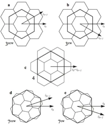
Research in multi-precision hexagonal lattices has focused on the three central place apertures (Dacey, 1965; Christaller, 1966), or ratios of cell area between each precision and the next coarser precision. These are apertures 3, 4, and 7, which are illustrated in figure 1. In the case of aperture 3, each finer precision grid can be constructed by uniform scaling by 1/√3 and rotating about the origin by 30° either clockwise or counterclockwise. Under aperture 4, finer precision grids are constructed by scaling by a factor of 1/√4 (or 1/2), with no rotation required. And for aperture 7 each finer precision grid can be constructed by scaling by 1/√7 and rotating about the origin by asin(√(3/28)) degrees (approximately 19.1°) either clockwise or counterclockwise.
Figure 1. Multi-precision hexagonal grids of aperture 3, 4, and 7 respectively.
The most useful linear spatial indexes for hexagonal cells can be constructed using hierarchical prefix codes, where each digit in the index corresponds to a location at a single precision relative to a hierarchical parent’s index. Such an indexing implicitly defines both a locality-preserving total ordering of the cells and a pyramid data structure, and enables the development of efficient hierarchical algorithms, making it ideal for use as a primary location spatial database key. The canonical example of a hierarchical prefix code is the square quadtree (Gargantini, 1982), where a square is recursively sub-divided into 4 smaller squares, each of which is assigned an index consisting of the parent square’s index concatenated with one of the digits 1, 2, 3, or 4. Hierarchical prefix location codes naturally encode both direction and precision, without the need for metadata, and provide an implicit algorithm for feature generalization via index truncation (Dutton, 1999). An arithmetic can be defined on these indexes using very efficient per-digit table lookups (Bell & Holroyd, 1991).
(GBT) (Gibson & Lucas, 1982), which generalizes one-dimensional balanced ternary addressing to the three natural axes of a hexagon grid. As illustrated in figure 3, in any seven-hex unit the central seven-hex is designated digit 0. The digits 1 through 6 are arranged so that, if the digits are stored as 3-bit binary values, digits on opposite sides of the central hex are binary complements of each other, allowing negation to be performed efficiently using the binary complement operation. Depending upon the application, the remaining unused possibility per 3-bit digit, octal digit 7, can be used to represent the aggregate group of seven child cells associated with the indexed cell (Gibson & Lucas, 1982), to efficiently indicate that the maximum known precision has been reached, or to indicate that all higher precision digits are zero, efficiently communicating with a finite number of digits that the index exactly represents the center point of the cell with infinite precision (Sahr, 2008; Sahr, 2011). Common vector operations, such as addition and scaling, have been defined on GBT using very efficient per-digit table lookups.
Figure 2. Central place children under all possible central place apertures: (a) aperture 3 with counterclockwise rotation; (b) aperture 3 with clockwise rotation; (c) Aperture 4; (d) aperture 7
with counterclockwise rotation; (e) aperture 7 with clockwise rotation.
Figure 3. CPI digit assignment at successive precisions, defined relative to the i-axis at that precision.
Since CPI children of a particular cell in aperture 3 and 4 systems also form a 7-hex unit, just as in the aperture 7 case, we can also apply the GBT indexing arrangement to create hierarchical indexing schemes for aperture 3 (Sahr, 2008; Sahr, 2011) and 4 systems. While this approach can be applied to grid systems with a single aperture, the introduction of a uniform
indexing system for all apertures allows us to construct grid sequences with mixed apertures as well. We call this approach to uniform indexing for pure and/or mixed aperture multi-precision hexagon systems Central Place Indexing (CPI) (Sahr, 2010). A CPI system specification consists of the following:
1. a connected set of precision 0 cells, referred to as the system’s base tiles, and
2. a sequence of apertures 3, 4, and/or 7 that define the topology of each finer precision in the system. In the case of apertures 3 and 7 directions of rotation must also be specified.
Individual applications can design CPI system specifications that provide precisions that are most useful to that application. Note that finer precision girds are geometrically produced using only uniform scaling and rotation about the origin. Therefore, given any two (or more) CPI system specifications defined on the same set of base tiles, a higher precision grid that participates in both hierarchies can always be constructed, with a total number of precisions no greater than the sum of the number of precisions in each of the two disparate systems, providing a common denominator CPI system that allows the performance of exact calculations involving indexes from any two or more CPI systems, though care must be taken to track the precision of results involving operands that are not exactly represented.
We have begun defining common operations on planar CPI systems. Implemented algorithms (Sahr, 2010) include forward and inverse quantization from/to cartesian coordinates, and CPI index equality, addition/translation, subtraction, and metric distance operations. Operations on CPI indexes are defined using per-digit table lookups, which are exact, efficient, and often composable.
3.2 Encoding Multi-Precision Quantization
Note that non-centroid CPI children under apertures 3 and 4 have multiple potential addressing parents. A unique hierarchical prefix code can be assigned to each cell at each precision by recursively aggregating the finer precision cells into groups of 3 or 4 cells (for apertures 3 and 4 respectively) that tile the plane, and consistently assigning digits at each precision, using a digit base determined by the aperture (Burt, 1980; Bell & Holroyd, 1991). White et al. (1992) noted that the aperture need not be consistent across all precisions; they developed a computer program that generates multi-precision grids using an aggregation tiling unit approach that allows for mixed-aperture sequences of grid precisions, thus providing finer control over the choice of grid precision and inter-cell spacing. CPI allows us to define and uniformly index aggregation schemes involving one or more tiling units (e.g., Sahr, 2008; Sahr, 2011).
Figure 4(a). Point locations P1 and P2 lie in different coarser precision cells (with indexes A and B respectively), but in the
same cell at the next finer aperture 3 precision. Assuming a clockwise aperture 3 change in precision the points would have multi-precision quantization indexes of A6 and B3 respectively.
Figure 4(b). Point locations P1 and P2 lie in different coarser precision cells (with indexes A and B respectively), but in the
same cell at the next finer aperture 4 precision. The points would have multi-precision quantization indexes of A4 and B3
respectively.
3.3 Self Describing Systems
Each of the central place apertures has a particular semantic expressiveness. Under all three central place apertures a CPI child is always introduced with the same center as the parent (but with higher precision). In the case of aperture 3, CPI children are also introduced centered on each of the parent cell’s vertices. If we take the utility digit 7 to indicate exact representation, then in an aperture 3 grid a coarse precision cell with index A has a center point that is exactly A7, and vertices that are exactly A17, A27, ..., and A67. An aperture 4 grid likewise allows the exact description of each of the cell edge midpoints, while aperture 7 grids allow for sub-frequency addressing of cell interior points.
Given the finest precision grid in a CPI system, the addition of two finer precisions of apertures 3 and 4 (in either order) creates a system that can exactly represent all center points, vertices, and edge midpoints in that grid. Adding an additional aperture 7 grid allows for the sub-frequency addressing of the internal region of each cell. This is illustrated in Figure 5. We call any grid that includes these additional precisions a 347-suffix system.
Figure 5. The addition of an aperture 3 grid precision in (a) allows each coarser precision cell vertex to be exactly represented. Assuming the central coarse precision cell has index A, it’s vertices are exactly A17, A27, ..., and A67. The addition of an aperture 4 grid in (b) likewise allows the exact representation of each of the cell edge midpoints. Adding a final aperture 7 grid in (c) allows for sub-frequency addressing of cell
interior points.
Inspecting the geometry for each central place aperture illustrated in figure 1 we note that, in each case, the center point, vertices, and edge midpoints of a precision i cell all correspond to either a center point, vertex, or edge midpoint of cells at the next finer precision i+1. Thus any precision r grid, where r > i+1, that exactly represents the precision i+1 cell center points, vertices, and edge midpoints will also exactly represent those of the precision i grid, regardless of the aperture. By induction we can conclude that the addition of an aperture 3 and 4 grid added to the maximum resolution of a CPI system will exactly represent the cell center points, vertices, and edge midpoints of cells at every precision in that system, allowing users to manipulate the geometry of the entire system using exact integer CPI calculations. We say that such a reference system is self describing, because it can exactly represent its own geometry.
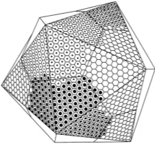
4. CONSTRUCTING AN OPTIMAL CPI DISCRETE GLOBAL GRID SYSTEM FOR VECTOR LOCATION Discrete global grid (DGG) systems (Sahr et al., 2003) are multi-resolution regular partitions of the earth’s surface into cells, often based on recursive partitions of the spherical platonic solids. We can extend planar CPI systems to the sphere to create a DGG system by tiling the spherical version of a regular polyhedra with CPI base tiles. The icosahedron is often chosen as the base polyhedra for DGGs because it has the smallest faces amongst the spherical platonic solids, which tends to minimize distortions in the system. When extending a CPI system to a spherical icosahedron special handling is required for tiles centered on the twelve icosahedral vertices, since these tiles will be pentagons at all precisions. For each pentagonal tile this can be accomplished by deleting one-seventh of the sub-hierarchy generated in the hexagon case, as described for the pure aperture 3 case in Sahr, 2008. That is, for a pentagonal base tile with address A all sub-cells are indexed as per a hexagonal base tile except that sub-cells with sub-indexes of the form AZd are not generated, where Z is a string of 0 or more zeroes and d is the sub-digit sequence (1, 2, 3, 4, 5, or 6) chosen for deletion. All hierarchical descendants of these deleted sub-cells are likewise not indexed. We should note that it has been claimed by some (e.g., Vince & Zheng, 2009) that a spherical mapping of the aperture 7 case is not possible; however application of our sub-digit deletion technique works for all three central place apertures, 3, 4, and 7 (see figure 6).
Figure 6. A portion of a precision 2 aperture 7 DGG system on an icosahedron constructed using sub-digit deletion.
symmetrical about both the equator and the prime meridian, ensuring that static data sets and dynamic simulations that use this system do not display inherent asymmetries between the traditional earth octants.
Figure 7. Base system spherical icosahedron oriented for octant symmetry.
We note that the north and south poles — as well as the intersection of the equator with the prime and anti-meridians — have exact representations in important real number reference frames (e.g., latitude/longitude, and the Centered, Earth-Fixed coordinate system) and are key point locations for many purposes. We therefore choose an aperture 4 grid for the first precision (see figure 8) so that our system can represent all of these important points exactly at any grid precision.
Figure 8. Cell boundaries for the aperture 4 first grid precision. Note the cell centered on the North Pole.
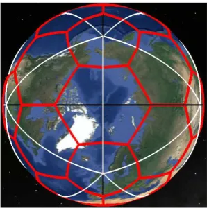
The vertices of the spherical icosahedron, along with the points at the center of each of the spherical icosahedral faces, form the vertices of the 120 icosahedral Least Common Denominator triangles (Fuller, 1975), any one of which can be used to reconstruct the entire icosahedron via symmetrical reflection; the introduction of these face center points captures the full icosahedral symmetries. We therefore choose aperture 3 for the second grid precision, which allows us to exactly represent these points (see figure 9). This yields 122 cells (110 hexagons and 12 pentagons), with an inter-point spacing of approximately 2,036 km. We choose these cells as the set of base tiles for our grid system and designate the resulting class of CPI DGG systemsCPI43 systems.
Figure 9. Two views of the CPI43 System base tile cell boundaries, generated on a spherical icosahedron using a grid
sequence of one aperture 4 followed by one aperture 3 grid precision.
We assign numeric values of 0 and 121 to the north and south pole-centered base tiles respectively, and assign values to the other 120 tiles so that they increase as they move south, roughly encoding relative latitude position in the base tile values. We note that the 122 base tile values can be stored uniquely using 7 bits, one short of an 8-bit byte. We use the low-order bit of that byte to indicate whether an address uses a 7 digit to indicate infinite precision (a value of 0), or the termination of a finite precision representation (a value of 1). The remaining bit values in an index encode digits in a particular CPI hierarchy centered on that base tile, with three bits per precision. Thus the north pole, for example, is encoded with infinite precision in all CPI43 systems as the 11-bit index 000000001112, independent
of the aperture sequence chosen for higher precision grids in a particular CPI43 system instance.
We can reduce the number of bits required to represent a location by introducing aperture 7 grids into our CPI sequence. Using only aperture 7 additional grids we can achieve 1-meter precision with 15 additional precisions beyond the base tile, for a total index size of 53 bits. Amongst the three apertures, aperture 7 grids also do the best job of maintaining the hexagonal topology of a base tile, so it would make sense to introduce aperture 7 grids at the coarsest precisions, introducing finer-grained aperture 4 and/or 3 precisions only when the desired spatial frequency regime is achieved. Note that doing so does mean that the resulting indices are only true multi-precision quantifiers within the finest (aperture 3 and/or 4) precisions of the system.
Finally, we should emphasize that the same planar CPI system advantages described above accrue to spherical CPI43 systems. Specifically, we can always exactly represent all system cell center points, vertices, edge midpoints, and cell interiors by the addition of a 347-suffix system. And since all CPI43 systems share the same set of base tiles, we can also always introduce a common denominator CPI system that will allow us to perform exact calculations involving indexes from any two or more CPI43 systems.
5. CONCLUSIONS AND DIRECTIONS FOR FURTHER RESEARCH
A systematic evaluation of the design requirements and alternatives for the fixed-width representation of point location, based purely on the criteria of representational and operational efficiency, and semantic fidelity, leads to the conclusion that the optimal known solution is a representation based on multi-precision mixed aperture hexagonal grids with a hierarchical integer indexing, and the most efficient known encoding for such systems is CPI. An examination of geometric considerations further led us to develop a specific class of spherical CPI systems, CPI43 systems. These systems meet our primary design criteria of multi-precision hexagonal point distribution, exact representation of key locations, and encoding of multi-precision quantization, as well as being self describing. We have successfully implemented key CPI operations on the plane and CPI43 grid generation on the sphere in prototype software. However, a more thorough quantitative evaluation of the efficiencies (and possible limitations) of such systems will require the definition and implementation of a more comprehensive set of vector CPI43 operations on the sphere.
6. REFERENCES
Android Open Source Project, 2013. Location Class Reference. http://developer.android.com/reference/android/location/Locatio n.html#getAccuracy() (September 9, 2013).
Apple Inc., 2010. CLLocation Class Reference. iOS Developer Library. hexagonally sampled binary images. Computer Graphics and Image Processing, 14, pp. 271–280.
Christaller, W., 1966. Central places in southern Germany. Prentice Hall, Englewood Cliffs, NJ.
Conway, J.H., Sloane, N.J.A., 2010. Sphere packings, lattices and groups. 3rd ed., Springer Verlag, New York, 703p.
Dacey, M.F., 1965. The geometry of central place theory. Geografiska Annaler: Series B, Human Geography, 47(2), pp. 111-124.
Dutton, G. 1999. A hierarchical coordinate system for geoprocessing and cartography. Berlin, Germany: Springer-Verlag. 231p.
Fuller R.B., 1975. Synergetics. New York: MacMillan, 876 pp.
Gargantini, I., 1982. An effective way to represent quadtrees. Communications of the Association for Computing Machinery, 25(12), pp. 905-910.
Gibson, L., Lucas, D., 1982. Spatial data processing using generalized balanced ternary. Proceedings of the IEEE Computer Society Conference on Pattern Recognition and Image Processing, Las Vegas, NV, pp. 566-571.
Goodchild, M.F., 2010. Twenty years of progress: GIScience in 2010. Journal of Spatial Information Science, 2010(1), pp. 3-20.
Goodchild, M.F., Guo, H., Annoni, A., Bian, L., de Bie, K., Campbell, F., Craglia, M., Ehlers, M., van Genderen, J., Jackson, D., Lewis, A.J., Pesaresi, M., Remetey-Fülöpp, G., Simpson, R., Skidmore, A., Wang, C., Woodgate, P., 2012. Next-generation digital earth. Proceedings of the National Academy of Sciences of the United States of America, 109(28), pp. 11088–11094.
Hayes, B., 2001. Third base. American Scientist, 89(6), pp. 488-492.
IEEE Computer Society, 2008. IEEE Standard for Floating-Point Arithmetic. IEEE Std 754-2008. 70p.
International Organization for Standardization (ISO), 2012. ISO 5725-6:1994 = Accuracy (trueness and precision) of measurement methods and results -- Part 6: Use in practice of accuracy values, 41p.
Kimerling, A.J., Sahr, K., White, D., Song, L., 1999. Comparing geometrical properties of global grids. Cartography and Geographic Information Science, 26(4), pp. 271-287.
Knuth, D., 2011. The art of computer programming; Volume 2: Seminumerical algorithms. Addision-Wesley, Menlo Park, CA, 762p.
Lalanne, L., 1840. Note sur quelques propositions
d'arithmologie elementaire. Comptes Rendus
Hebdomadaires des Seances de l'Academie des Sciences, 11, pp. 903-905.
Olea, R.A., 1984. Sampling design optimization for
spatial functions. Mathematical Geology, 16(4), pp.
369-392.
N-dimensional Euclidean spaces. Information Control, 5, pp. 279-323.
Rogers, C.A., 1964. Packing and Covering. Cambridge University Press, 111p.
Saff, E.B., Kuijlaars, A., 1997. Distributing many points on a sphere. Mathematical Intelligencer, 19(1), pp. 5-11.
Sahr, K., White, D., Kimerling, A.J., 2003. Geodesic discrete global grid systems. Cartography and Geographic Information Science, 30(2), pp. 121–134.
Sahr, K., 2008. Location coding on icosahedral aperture 3 hexagon discrete global grids. Computers, Environment and Urban Systems, 32(3), pp. 174-187.
Sahr, K., 2010. Central Place Indexing Systems, U.S. Patent Application 2010/054550.
Sahr, K., 2011 (awarded), Icosahedral Modified Generalized
Balanced Ternary and Aperture 3 Hexagon Tree, US Patent
#07,876,967.
Vince, A., Zheng, X., 2009. Arithmetic and Fourier transform for the PYXIS multi-resolution digital earth model. International Journal of Digital Earth, 2(1), pp. 59-79.
White, D., Kimerling, A.J., Overton, W.S., 1992. Cartographic and geometric components of a global sampling design for environmental monitoring. Cartography and Geographic Information Systems, 19(1), pp. 5-22.
Yu, L., Gong, P., 2012. Google Earth as a virtual globe tool for Earth science applications at the global scale: progress and perspectives, International Journal of Remote Sensing, 33(12), pp. 3966-3986.
7. ACKNOWLEGEMENTS