Published online 26 March 2010 in Wiley Online Library (wileyonlinelibrary.com). DOI: 10.1002/nme.2880
Least-square-based radial basis collocation method for solving
inverse problems of Laplace equation from noisy data
Xian-Zhong Mao
∗,†and Zi Li
Research Center for Environmental Engineering and Management,Graduate School at Shenzhen,
Tsinghua University,Shenzhen 518055,People’s Republic of China
SUMMARY
The inverse problem of 2D Laplace equation involves an estimation of unknown boundary values or the locations of boundary shape from noisy observations on over-specified boundary or internal data points. The application of radial basis collocation method (RBCM), one of meshless and non-iterative numerical schemes, directly induces this inverse boundary value problem (IBVP) to a single-step solution of a system of linear algebraic equations in which the coefficients matrix is inherently ill-conditioned. In order to solve the unstable problem observed in the conventional RBCM, an effective procedure that builds an over-determined linear system and combines with least-square technique is proposed to restore the stability of the solution in this paper. The present work investigates three examples of IBVPs using over-specified boundary conditions or internal data with simulated noise and obtains stable and accurate results. It underlies that least-square-based radial basis collocation method (LS-RBCM) poses a significant advantage of good stability against large noise levels compared with the conventional RBCM. Copyright q 2010 John Wiley & Sons, Ltd.
Received 28 November 2008; Revised 26 January 2010; Accepted 31 January 2010
KEY WORDS: inverse problems of Laplace equation; radial basis collocation method; least-square technique; noise levels
1. INTRODUCTION
In many practical situations, the known boundary data are not complete due to technical difficulties associated with measurement and acquisition of accurate data. For example, a part of boundary is inaccessible to direct measurement, or the presence of measuring devices disturbs the physical process under investigation. Even the location of boundary itself is sometimes unknown resulting
∗Correspondence to: Xian-Zhong Mao, Research Center for Environmental Engineering and Management, Graduate
School at Shenzhen, Tsinghua University, Shenzhen 518055, People’s Republic of China.
†E-mail: [email protected]
Contract/grant sponsor: SRF for ROCS, SEM
from special geological features. Therefore, the inverse boundary value problem (IBVP) arises to deal with the estimation of the recovered boundary conditions on unspecified part of the boundary. In order to make the problem solvable, partial accessible boundary may be over-specified; for example, the Dirichlet and the Neumann conditions are simultaneously prescribed, in some cases the auxiliary internal data are necessary for input.
The IBVPs arise from many engineering applications such as heat transfer [1], geophysical prospecting[2], medical imaging and non-destructive testing[3]and acoustic and electromagnetic waves[4]. It is well known that the inverse problems have a typical characteristic of ill-posedness in the sense that a slight error in the input data may produce an enormous change in the output solution that makes them more difficult to deal with. However, the measurement inevitably poses some noises due to the technical and physical difficulties. It is required to develop a numerical method to solve the inverse problem with noisy data input.
Traditional methods, such as finite difference method (FDM), finite element method (FEM), finite volume method (FVM) and boundary element method (BEM), have been proposed for these kinds of inverse problems, which require to combine with special optimization schemes to solve the direct problems through iterative procedure till the convergent solution is obtained. Essentially they need a mesh on the domain to support the solution process, which will cost large consuming time for generating a good quality mesh for complicated geometry, especially in high dimensions. Although the BEM reduces the dimensionality of the problem and partially alleviates the difficulty, it requires the evaluation of singular integrals for using singular fundamental solutions, and employing an iterative BEM based on regularization algorithm to obtain the convergent solutions in the inverse Laplace problems[5, 6].
In recent years, meshfree methods (MMs), including the method of fundamental solutions (MFS)
[7], the boundary knot method (BKM)[8]and the radial basis collocation method (RBCM) [9], emerged as competitive alternatives to the traditional methods due to their meshfree and non-iterative characteristics for the inverse problems. All of the MMs directly induce the inverse problem to a single-step solution of a system of linear algebraic equations. However, the MFS is a versatile boundary-type meshless numerical scheme and free from treatment of singularities since the source points are always placed outside the domain. It has been successfully applied to the inverse heat conduction problem [10], backward heat conduction problem [11], Cauchy problem associated with Helmholtz-type equation[12]and Cauchy problem of Laplace equation
No matter which MM is adopted, the inverse problems can be converted to a large-scale system of linear algebraic equations in which a number of unknown coefficients need to be determined. However, the coefficient matrix is inherently ill-conditioned and the solution is highly sensitive to the noise of measured input data. Many regularization methods are additionally employed to obtain stable solutions, for example, the standard Tikhonov regularization (TR) technique with the L-curve criterion (LC)[10–12], the truncated singular-value decomposition (TSVD) with the LC[15]and three regularization strategies (TR, TSVD and damped singular-value decomposition) under the different choices for the regularization parameter[14]. Although Li[17, 18]and Cheng and Cabral[19] achieved some encouraging results through the RBCM, they did not test the bad conditioning of the coefficient matrix that may cause the unstable results from noisy data input.
In this paper, we apply the least-square-based RBCM to the inverse problems of Laplace equation with noisy data input. In the proposed approach, an over-determined linear system of algebraic equations is constructed and the least-square procedure is naturally necessary to obtain the stable solution. This paper is organized as follows. Section 2 describes the mathematical formulation of inverse Laplace problems. Section 3 presents the least-square-based radial basis collocation method (LS-RBCM), and its adaptation to the problem is discussed. Section 4 tests the proposed methodology and compares with the conventional RBCM using three examples. The numerical examples include the problem of under-specified boundary recovered from internal data, identification of missing boundary condition from over-specified boundary conditions and shape identification problem. And the sensitivity of the LS-RBCM method with respect to the shape parameter and mesh size is investigated. Finally, the conclusion is given in Section 5.
2. INVERSE PROBLEMS FOR THE LAPLACE EQUATION
The mathematical formulation of the 2D Laplace equation, as the governing equation for a field potential or steady-state heat conduction problem defined in a domainbounded by a surface, is defined by the following expression:
∇2u=0 in⊂R2 (1)
And partial boundary condition is given by
u=f on1∈ (2)
whereuis the potential or temperature to be solved and f is the prescribed boundary condition on1 that is usually only a part of the whole boundary. The necessary information on another
part boundary2 with2=Ø and 1+2= is not available. Then the IBVP arises to recover
the boundary value on2 or restore the shape of boundary 2. If the inverse problem holds, it
is necessary to add other conditions together with Equation (2) to make Equation (1) identifiable. Two types of inverse problem arise subject to the different conditions.
If the following boundary condition is given:
*u
*n=g on 1∈ (3)
in which,g is the prescribed fluxes on 1, the problem described by Equations (1)–(3) is the
over-specified, and 2 is under-specified. Equation (3) compensates for the missing boundary
condition on2. The Cauchy problem for the Laplace equation arises from many fields in science
and engineering, such as non-destructive testing [20], steady-state inverse heat conduction [21]
and electro-cardiology[22].
The prescribed data f and fluxesgcan be provided on partial accessible boundary1by physical
measurement that inevitably contains certain level noises. The Cauchy problem is very difficult to be solved both numerically and analytically since the solution does not depend continuously on the prescribed boundary conditions[23].
Another inverse problem needs the assistance of the following auxiliary internal information together with Equation (2) to make Equation (1) solvable:
u=h in Q∈ (4)
whereh is the prescribed data on the set Q in the domain. Internal potential or temperatureh can be measured at some interior locations instead of fluxes on1 to stabilize the solution. The
problem presented by Equations (1), (2) and (4) is another commonly used inverse problem in the Laplace equation.
3. LEAST-SQUARE-BASED RADIAL BASIS COLLOCATION METHOD
3.1. The RBCM
The RBCM is one of MMs to solve IBVPs, which does not require the discretization of compu-tational domain and is independent of fundamental or general solution to particular differential operators. In RBCM, the numerical solution for the potential or temperature is approximated by the following linear combination of radial basis functions:
u(x)=
m
k=1
k(x,xk)k (5)
where m is total number of the collocation points distributed in two-dimensional domain; xk denotes spatial coordinates of collocation points;k represents the coefficient to be determined by the collocation method using the governing equation and the prescribed boundary conditions; k(x,xk)is radial basis function. In the present work, the IMQ is chosen as RBF
k(x,xk)=(c2+x−xk2)−1/2 (6)
where the distancex−xkis usually taken to be the Euclidean metric;cis a constant referred as the shape parameter, which leads to the scheme’s exponential convergence property. Hardy[24], Kansa and Carlson[25]and Golberg et al.[26]provided some useful guidelines of determining the optimal shape parameter.
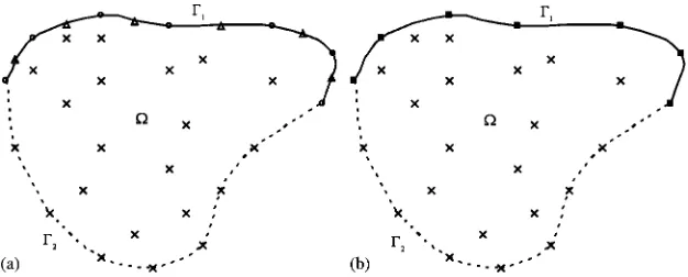
Taking the Cauchy problem for example, we can use Figure 1 to illustrate how RBCM obtain a system of linear algebraic equations to solve the inverse problem of Equations (1)–(3). As shown in Figure 1, the problem is defined in a domainbounded by the known boundary1(solid line)
and unknown boundary2 (dashed line). The geometrical configuration with the distribution of
Figure 1. Distribution of collocation points in the conventional RBCM (a) and LS-RBCM (b) for the Cauchy problem.
Table I. Different symbols denoting different collocation points satisfying the corresponding conditions.
The symbol The condition(s) satisfied
× The governing equation
◦ The Dirichlet conditions
△ The Neumann conditions
The Dirichlet and the Neumann conditions
• The Dirichlet conditions and governing equation
The Neumann conditions and governing equation
The Dirichlet and the Neumann conditions, and governing equation
As shown in Figure 1(a), there aren1interior points (including points on unknown boundary2)
shown in × symbol satisfying the governing equation only, n2 points on the known boundary 1 shown in ◦ symbol satisfying the Dirichlet conditions only and n3 points on the known
boundary1 shown in △symbol satisfying the Neumann conditions only. Totally there are m=
(n1+n2+n3)collocation points in the conventional RBCM. By substituting Equation (5) into the
governing equation (1) and the prescribed boundary conditions (2) and (3), and collocating on the corresponding points, we are able to obtain the following well-determined system of linear algebraic equations:
m k=1
∇2k(xi,xk)k=0, i=1, . . . ,n1, xi∈ (7)
m
k=1
k(xi,xk)k=f(xi), i=n1+1, . . . ,n1+n2, xi∈1 (8)
m k=1
*
k(xi,xk)
Equations (7)–(9) form a linear system of(n1+n2+n3)equations withm(=n1+n2+n3)unknown
coefficients, which can be written in the following form:
[Ai k][k] = [bi] (10)
where[k]is the unknown coefficient;[Aik]is the resultant square coefficients matrix; [bi]is the column vector that contains the prescribed boundary conditions. The coefficients matrix and the right-hand column vector are expressed as
[Aik] =
If the square matrix [Aik]is non-singular, the solution of Equation (10) can be solved by the Gaussian elimination method[16], the Linpack’s Cholesky decomposition [13] or LU decompo-sition solver[17].
especially when the input contains large noise. Kee et al. [27] believed that such oscillation is caused by the strong requirement for the approximated field variable to satisfy governing equation and boundary conditions exactly at all the nodes. They have further found that the Neumann boundary condition is the cause of the instability. It could be due to the ‘strong’ requirement of satisfaction of the Neumann boundary condition in the strong formulation.
To provide a kind of ‘relaxation’ effect, we employ the double boundary collocation approach
[28] and the double use of boundary collocations[8]to construct an over-determined system for Equation (10) and combine with least-square method to stabilize the solutions for the 2D inverse Laplace problems. The double boundary collocation approach [28] requires that the governing equation is collocated at all the collocation points in the domain, including on the boundary, namely the collocation points on the boundary satisfy not only the boundary conditions, but also the governing equation. The resultant coefficients matrix is still well-determined in[28]. The double use of boundary collocations [8] requires the Dirichlet conditions and the Neumann conditions collocating on the same nodes of the boundary. Compared with the conventional RBCM, two types of collocation points are used in the present RBCM: on totalmpoints in the whole domain (shown in × symbol, and in symbol in Figure 1(b)), the governing equation is collocated using the double boundary collocation approach; and onnpoints of the over-specified boundary1(shown
insymbol in Figure 1(b)), both the Dirichlet and the Neumann conditions are collocated with the double use of boundary collocations. Hence by the governing equation collocating onmpoints in the whole domainand both the Dirichlet condition and the Neumann condition collocating onnpoints of the over-specified boundary1, we are able to have an over-determined system of
linear algebraic equations.
With the new collocation approach, [Aik] becomes a rectangular coefficients matrix in the system of linear algebraic equations (10), which hasm unknown coefficients to be determined in (m+2n) linear equations system. Equation (10) is an over-determined system with m+2n>m. This aims to relax the ‘strong’ requirement of satisfaction of the governing equation and boundary conditions to improve the conditioning of the coefficient matrix and the solution accuracy. For an over-determined system (10), the least-square method can provide a best-fit approximation to the solution.
3.2. Least-square technique using the singular-value decomposition(SVD)with rank reduction
The unknown coefficients [k] in (10) can be determined by minimizing L2 norm using the
least-square method in the following over-determined system:
min{A−b2} (11)
The least-square problem of Equation (10) can be solved using QR-algorithm[27]. In the present process, the singular-value decomposition (SVD) is applied to find the solution to the least-square problem. The matrix[Aik]is decomposed using the SVD method as follows:
A=
m
k=1
kukvTk (12)
Using the SVD of matrix A, it is straightforward to show the ordinary least-squares solution to Equation (10).
ls=
m
k=1
uTkb
k
vk (13)
Because the over-determined system (10) from the discrete ill-posed problem is still ill-conditioned and the condition number shown as
CDN=1
m (14)
is extremely large, the error in the directions corresponding to smaller singular values is greatly magnified and overwhelms the information contained in the directions corresponding to larger singular values due to the error present in the vectorb[29]. Hence, we should filter out enough noise without losing too much information in the computed solution by finding a good regularization parameter that controls how much filtering is introduced.
In our computation, the SVD with rank reduction [30] is employed to regularize the solution and the regularization parameter is in essence the tolerance whose value defaulted in theMatlab code is
=max[size(A)]·norm(A)·eps (15)
where max[size(A)] is the maximum one of (m+2n) and m; norm(A) is the 2-norm of matrix A, which is presented by the largest singular value1; eps is the floating-point relative accuracy.
By treating any singular value less than the tolerance as zero, we reduce the full rank m to the effective rankr with1· · ·rr+1· · ·m and obtain the regularization solution of
Equation (11).
reg=
r
k=1
uTkb
k
vk (16)
The objective of this paper is to illustrate the advantage of the LS-RBCM in aspects of stability and accuracy against larger noise level in contrast with the conventional RBCM. For comparison, the square coefficient matrix[Aik]resulted from the conventional RBCM is also solved using the solution (16) in the numerical examples.
The capability of the LS-RBCM to resist the noises will be demonstrated numerically in the following sections. And accuracy and stability of the LS-RBCM are also discussed.
4. NUMERICAL EXAMPLES
For simplicity, we use random noise simulating the measurement noise in the numerical examples. The simulated noisy data is generated by
i=i[1+e·rand(i)] (17)
level is similar for different random noises. For comparison, we choose only one group of random noise for each example.
The accuracy of the numerical solution to verify the efficiency and the stability of the proposed method is measured by the following relative root mean square error (RRMSE):
RRMSE=
1 N
N
j=1[ua(xj)−un(xj)]2
1 N
N
j=1ua(xj)2
(18)
where{xj} is the set of test points; N is total number of test points;ua(xj)and un(xj)are the analytical solution and numerical solution at the test points, respectively. In our computation, we take N=21 and{xj}is uniformly distributed on the boundary.
4.1. Problem with under-specified boundary condition and internal data
Onishi [31] investigated the ill-posed Laplace problem of potential flow on a square domain
[0,3]×[0,3], which has the following exact solution:
u(x,y)=x2−y2 (19)
and the Dirichlet conditions prescribed on the left, top, and right sides of boundary as follows:
u(0,y)= −y2, u(x,3)=x2−9, u(3,y)=9−y2 (20)
No boundary condition is given on the bottom side. Obviously, the problem is not identifiable unless sufficient measurement data in the interior points are supplied. The internal potential values on four points are given based on the exact solution
u(1,1)=0, u(1,2)= −3, u(2,1)=3, u(2,2)=0 (21)
for compensation to numerically identify the Dirichlet condition on the bottom side of boundary
u(x,0)=x2 (22)
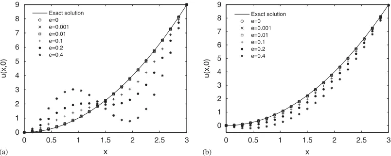
Cheng and Cabral[19]investigated the numerical example, and reported that the accuracy of RBF solution is somewhat better than the FEM solution in[31]with the relatively sparse mesh 7×7. No noise was considered for input data.
In the present work, the simulated noises are imposed with different levels from 10−3to 0.4 on
the internal potential values in Equation (21). For comparison, the distribution of collocation points for the conventional RBCM and LS-RBCM is shown in Figure 2 and the collocation points are distributed on a 7×7 grid too. The collocation points are represented by different types of symbols satisfying the corresponding conditions as listed in Table I. It also needs to select a proper valuec for IMQ function in Equation (6), and we choosec=4 as Cheng and Cabral[19]recommended.
Figure 2. Distribution of collocation points in the conventional RBCM (a) and LS-RBCM (b).
Figure 3. The recovered u(x,0) with different noise levels in the conventional RBCM (a) and LS-RBCM (b).
whereas the error from the conventional RBCM is greater than 48.8%, and the approximation curve is deteriorated, as shown in Figure 3(a).
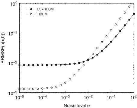
Figure 4 shows the RRMSE distribution of both methods against different noise levels. An attractive phenomenon is observed that there exists a critical point at noise level e=0.01, which fully shows different advantages for both methods in different noise ranges: when the noise level e<0.01, the solutions of conventional RBCM are better; whereas when the noise level e>0.01, the solutions of LS-RBCM are much better than the ones of conventional RBCM.
We also observe from Figure 4 that the input with small noise (less than 10−4) can match the
100 100
Noise level e
RRMSE(u(x,0))
RBCM
Figure 4. The RRMSE of recoveredu(x,0)against noise level in the conventional RBCM and LS-RBCM.
the solution depends only on the method of RBCM, not the noise. When the noise level is greater than 10−3, the RRMSE is proportional (very sensitive) to the noise level, and the accuracy depends
on the noise only. Under the large noise-level condition, this ‘strong’ requirement may cause the solution distorted as shown in Figure 3(a).
However, LS-RBCM provides ‘relaxation’ effect for the requirement, which aims to search for a best-fit approximation to the solution in a new-constructed over-determined system. The solution of LS-RBCM is not sensitive to the noise tille=0.01, and if noise level is greater than 0.01, the RRMSE is proportional (sensitive) to the noise level. Fortunately, the gradient of RRMSE curve is relatively smaller, and the solution is still a best-fit one as shown in Figure 3(b). The numerical solutions from the input with larger noise are under-estimated since it might be caused by bias of the random noise chosen only if four points are used.
It illustrates that ‘relaxation’ effect in LS-RBCM strengthens the stability of the solution and improves the accuracy to resist the large noise levels, but somewhat sacrifices the accuracy of the numerical solution within the smaller noise levels. The over-determined system improves ill-conditioning of the coefficient matrix and the condition number defined by Equation (14) decreases from 1.68×10¹¹in conventional RBCM to 9.39×10⁹ in LS-RBCM.
0 0.5 1 1.5 2 2.5 3 0
1 2 3 4 5 6 7 8 9
x
u(x,0)
Exact solution e=0 e=0.001 e=0.01 e=0.1 e=0.2 e=0.4
Figure 5. The recoveredu(x,0)with eight internal data in LS-RBCM.
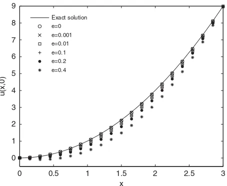
In order to test the sensitivity of the solution to the input information, we further provide the internal data on four additional points as follows:
u(1,1.5)= −1.25, u(1.5,2)= −1.75, u(2,1.5)=1.75, u(1.5,1)=1.25 (23)
The input is also contaminated by the noise. Hence, we have four additional collocation points. It requires that four additional linear algebraic equations are included in the system (10), whereas the number of unknown coefficients remains constant (still based on the 7×7 grid). The numerical solutions and the RRMSE distribution are shown in Figures 5 and 6, respectively. The RRMSE of recovered u(x,0) with eight interior nodes input is always smaller for all noisy levels. The RRMSE curve shifts 30–40% downward as shown in Figure 6 and the recoveredu(x,0)is better fit to the exact one as shown in Figure 5. It means the better the solution of LS-RBCM is with more input information at the same noise level, even the input is contaminated with larger noise. When the noise level is 40%, the RRMSE is reduced to 13.8 from 18.1%. It is quite encouraging for practical applications. The targeted solution can be achieved at the cost of more collecting data.
100
Noise level e
RRMSE(u(x,0))
4 internal nodes 8 internal nodes
Figure 6. The RRMSE of recoveredu(x,0)with four and eight internal data in LS-RBCM.
0 2 4 6 8 10 12
100
c
RRMSE(u(x,0))
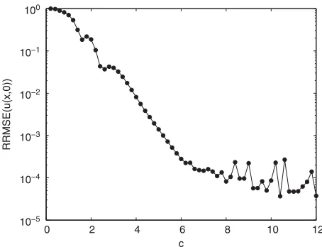
Figure 7. The RRMSE of recoveredu(x,0)in LS-RBCM with different valuec.
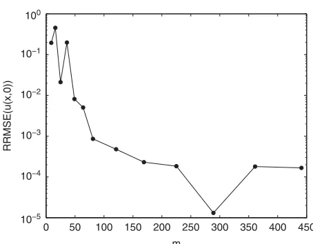
the results in Figure 8 are obtained for a fixed shape parameter c=4, which should not be the optimal one for different mesh sizes.
4.2. Problem with over-specified boundary condition
Lesnicet al.[5]considered the following ill-posed Cauchy problem of heat conduction on a square domain [0,1]×[0,1] with the over-specified boundary condition on partial boundary. The exact solution of the Laplace equation is
0 50 100 150 200 250 300 350 400 450 100
m
RRMSE(u(x,0))
Figure 8. The RRMSE of recoveredu(x,0)in LS-RBCM with different collocation meshm.
The boundary condition is missing on one side of the domain. It assigns the Dirichlet condition, the Neumann condition, and both the Dirichlet and the Neumann conditions on the bottom, top and right sides of the boundary based on the exact solution (24), respectively.
u(x,0)=cos(x) (25)
*u(x,1)
*y =cos(x)sinh(1)+sin(x)cosh(1) (26)
u(1,y)=cos(1)cosh(y)+sin(1)sinh(y) (27)
*u(1,y)
*x = −sin(1)cosh(y)+cos(1)sinh(y) (28)
The Cauchy problem arises to recover the following Dirichlet and the Neumann conditions on the left-side boundary:
u(0,y)=cosh(y) (29)
*u(0,y)
*x =sinh(y) (30)
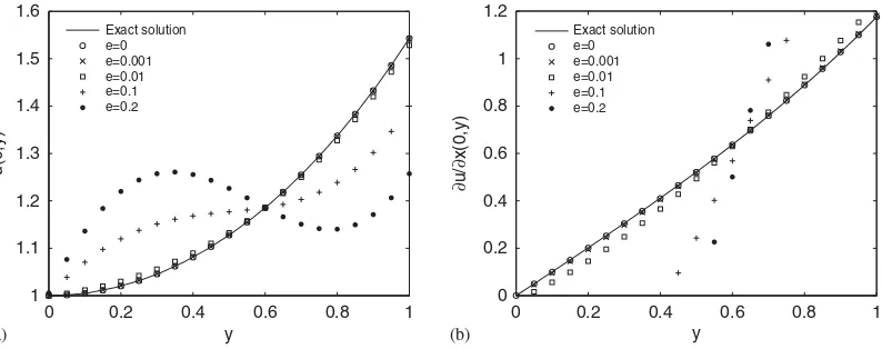
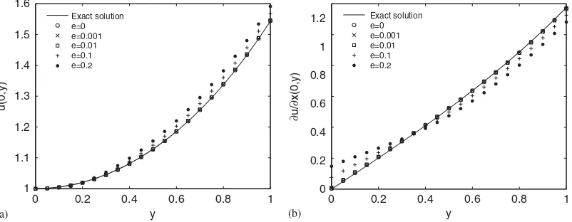
Younget al.[13]used the double precision MFS to solve the temperature and heat flux distri-butions on the missing boundary. It showed that the results had good agreement with the exact solution when boundary conditions were imposed with noise level from 10−5 to 10−3, and when larger noise 0.01 was used, regularization was necessary. Cheng and Cabral[19]showed the high accuracy using RBCM on different grid sizes from 6×6 to 12×12, but no noise was considered.
Figure 9. Distribution of collocation points in the conventional RBCM (a) and LS-RBCM (b).
In this example, we impose the simulated noise on the Cauchy boundary conditions (27) and (28). The shape parameter in IMQ is chosen asc=4.
The recovered solutionu(0,y)and fluxux(0,y)on the missing boundary with different noise levels using both methods are plotted in Figures 10 and 11. The RRMSE distribution against the different noise levels is shown in Figure 12. Similar phenomenon is observed as in Example 1, but the critical noise value moves to 0.001. When the noise level is smaller than 0.001, the solutions u(0,y)and fluxux(0,y)on the missing boundary of the conventional RBCM are better than the ones of LS-RBCM; whereas when the noise level is greater than 0.001, the solutions and flux of LS-RBCM are much better. When noise level reaches 20%, the RRMSEs of the temperature and heat flux on the left-side boundary in the conventional RBCM are about 14.7 and greater than 100%, and numerical curve is distorted as shown in Figure 10; while errors reduce to only 6.9 and 22.3% for the solution and flux in LS-RBCM, respectively, as shown in Figure 11.
Compared with Example 1, the Cauchy boundary problem poses high ill-conditioning of the coefficient matrix[Aik], which may result in the solution more sensitive to the noise. In the conventional RBCM, the over-specified boundary condition with very slight noise can match the ‘strong’ requirement to satisfy boundary conditions exactly at the collocation points. We observe from Figure 12 that the RRMSE of the solution and its flux are almost proportional (very sensitive) to the noise level even when the noise level is as small as 0.0001. The accuracy of the method depends on the noise level. However, the solution of the LS-RBCM is not sensitive to the noise level tille=0.001 and the flux is not sensitive to the noise level tille=0.004 due to ‘relaxation’ effect. Only when noise level is greater than 0.002 (0.005), the RRMSE of the temperature (flux) is proportional (sensitive) to the noise level. The gradients of RRMSE curves of the solution and its flux are expected to be smaller in LS-RBCM. And the RRMSE curve moves 55% downward of the temperature and 90% downward of heat flux when the noise levele>0.005.
0 0.2 0.4 0.6 0.8 1 levels in the conventional RBCM.
0 0.2 0.4 0.6 0.8 1
the accuracy to resist the noise levels, but somewhat sacrifices the accuracy of the numerical solution within the smaller noise levels.
100 in the conventional RBCM and LS-RBCM.
0 0.2 0.4 0.6 0.8 1
ux(0,y). That means, the better the solution of LS-RBCM is with more input information, even the input is contaminated with larger noise. When the noise level is up to 20%, the RRMSEs are reduced from 6.9 to 2.9% foru(0,y), and from 22.3 to 12.3% for the fluxux(0,y). The numerical solution and its flux are better fit to the exact ones with the more measured information input on the Cauchy boundary, as shown in Figure 13.
100 100
100 100
Noise level e Noise level e
RRMSE(u(0,y))
9 boundary nodes 17 boundary nodes
RRMSE(
∂
u/
∂
x(0,y))
9 boundary nodes 17 boundary nodes
(a) (b)
Figure 14. The RRMSE of recoveredu(0,y)(a) and ux(0,y) (b) with 9 and 17 boundary nodes input in LS-RBCM.
0 2 4 6 8 10 12
100 101
c
RRMSE
u(0,y)
∂u/∂x(0,y)
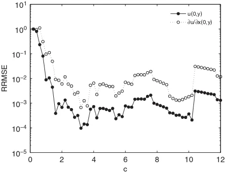
Figure 15. The RRMSE of recoveredu(0,y)andux(0,y)in LS-RBCM with different valuec.
4.3. Shape identification problem
Hon and Wu [16] investigated the following ill-posed problem for shape identification, which often arises in practical applications of non-destructive testing. The domain of interest is an upper half-plane. It is assumed that observation can be only conducted on a finite segment
{−0.5x0.5;y=0}of the boundary for the Cauchy conditions as follows:
u(x,0)=x2−0.31x−1.089 (31)
*u(x,0)
0 50 100 150 200 250 300 350 400 450 100
101
m
RRMSE
u(0,y)
∂u/∂x(0,y)
Figure 16. The RRMSE of recovered u(0,y) and ux(0,y) in LS-RBCM with different collocation meshm.
The problem is to search for the location of the internal shape that satisfies zero potential condition with the over-specified boundary condition on a segment of the boundary. The exact solution of the Laplace equation is
u(x,y)=(x−0.1)2−(y−1.1)2+0.1(x−0.1)(y−1.1)+0.1 (33) The problem is solved in finite domain [−2,2]×[0,2] due to the instability of the Cauchy condition and the constraint of finite range of the available data. The exact positions of the trajectories where the potential valueu(x,y)=0 is satisfied are
y=1.095+0.05x+1.0010.1098−0.2x+x2 (34)
y=1.095+0.05x−1.0010.1098−0.2x+x2 (35)
Hon and Wu[16]tested the sensitivity of solution subject to noisy boundary data from 10−5to
10−4. Eleven data points were used for collocation on the Cauchy boundary[−0.5,0.5]. When the
noise reached 10−4, the shapes became unidentifiable, and the solution failed. Cheng and Cabral [19]re-examined the numerical experiment using the RBCM on 9×9 grid, and collocated for the Dirichlet and the Neumann conditions each at five points on the Cauchy boundary. They found that when noise level was up to 0.01, the solution of lower trajectory started to deteriorate, but failed for the upper one. And they recovered the shape much improvingly with auxiliary information with one internal point. Younget al. [13] applied the MFS to investigate the problem, and collocated for the Dirichlet and the Neumann conditions each at six points on the Cauchy boundary. The zero potential result showed good accuracy when low noise level (10−5 to 10−3) was considered. However, for large values of noise level such as 0.01, regularization was necessary since the MFS would not give promising results in the upper branch.
Figure 17. Distribution of collocation points in the conventional RBCM (a) and LS-RBCM (b).
marked by different types of symbols (as listed in Table I) to satisfy the corresponding conditions. We impose the simulated noise on the Cauchy boundary conditions (31) and (32). The shape parameter in IMQ is chosen asc=4.
In our computation, we use Newton’s iteration method to search for the locations of the zero potential trajectories after the solution is obtained. The zero potential trajectories with different noise levels using the conventional RBCM and LS-RBCM are plotted in Figure 18, and the RRMSE distribution of the position along the different noise levels is plotted in Figure 19. The results show that we recover the lower branch very well, but there is a slight deviation for the upper one for both methods, and we cannot recover the upper branch when noise level is 0.01 in the computational region. And also we observe in Figure 19, LS-RBCM has much better results for both branches when noise is smaller e<10−4; however, when the noise goes to 0.01, the error tends to be of
the same magnitude for both methods till the computation fails to recover the upper trajectory at the noise levele=0.0063. The RRMSE of recovered solution on the top and bottom sides of the boundary in LS-RBCM is better than that in the conventional RBCM within small noise levels, as shown in Figure 20. The phenomenon is totally different from Examples 1 and 2. Why does LS-RBCM obtains better results than the conventional RBCM within small noise levels?
The Cauchy problem on a finite segment of boundary is extremely ill-posed. The input data with small errors will cause the solution to deteriorate rapidly. In the present work, a finite domain
0 1 2 0
0.5 1 1.5 2
x
y
Exact solution e=0 e=0.001 e=0.002 e=0.005 e=0.01
2
0 1
0 0.5 1 1.5 2
x
y
Exact solution e=0 e=0.001 e=0.002 e=0.005 e=0.01
(a) (b)
Figure 18. The recovered trajectories in the conventional RBCM (a) and LS-RBCM (b).
Noise level e
RRMSE
Upper for RBCM
Lower for RBCM
Figure 19. The RRMSE of recovered trajectories in the conventional RBCM and LS-RBCM.
In the conventional RBCM, the Dirichlet and the Neumann conditions are satisfied on two types of collocation points (total 10 points) as shown in Figure 17(a), whereas the Dirichlet and the Neumann conditions are satisfied simultaneously on the same five collocation points in LS-RBCM, as shown in Figure 17(b). The conventional RBCM can match ‘strong’ requirement to satisfy the Dirichlet and the Neumann conditions exactly on the corresponding nodes of the boundary; however, the Cauchy conditions in the problem are constrained only in a finite segment
100
Noise level e
RRMSE
Top for RBCM
Bottom for RBCM
Figure 20. The RRMSE of recoveredu(x,0)(bottom side) andu(x,2) (top side).
finite segment. This may be the reason why the RRMSE of both recovered trajectories and the RRMSE of the solutions on the top and bottom sides of boundary in LS-RBCM are much better than that in the conventional RBCM whene<0.001, then tends to the same RRMSE as the noise level increases till fails to recover the upper trajectory, as shown in Figures 19 and 20. In the conventional RBCM, the solutions of the top and bottom boundaries are not sensitive to the noise when e<0.002; however, the error of the solution on the top side boundary is as large as 15%, and the RRMSE of the solution on the top and the bottom sides of boundary is smaller than the one in LS-RBCM whene>0.003. The reason that the solutions on the bottom boundary and the lower trajectory are recovered much better is because the Cauchy boundary is a part of the bottom side of boundary.
We use four more points on the Cauchy boundary, namely total nine points are uniformly distributed on the boundary. The input is also contaminated by measurement noise. It requires that eight additional linear algebraic equations (four satisfying the Dirichlet condition, and another four satisfying the Neumann condition) are included in the system (10), whereas the unknown coefficients keep constant (still based on the 9×9 grid). The recovered trajectories of both branches are plotted in Figure 21, and the RRMSE distribution of the positions of the trajectories is shown in Figure 22. The RRMSE of the recovered solution on the top and the bottom sides of boundary is plotted in Figure 23. It is very encouraging that, only with four additional points as input, we successfully produce a reasonable approximation for the solution, and can recover the trajectories of both branches when the noise level goes to 0.1. The results are improved much better when the noise is greater than 10−4. Also we observe that when the noise level is less than 0.004,
0 1 2 0
0.5 1 1.5 2
x
y
Exact solution e=0 e=0.001 e=0.01 e=0.05 e=0.1
Figure 21. The recovered trajectories with nine boundary nodes input in LS-RBCM.
Noise level e
RRMSE
Upper for 5 boundary nodes Upper for 9 boundary nodes Lower for 5 boundary nodes Lower for 9 boundary nodes
Figure 22. The RRMSE of recovered trajectories with five and nine boundary nodes input in LS-RBCM.
from five points input, the errors of the solution and the position of trajectories on both sides drop dramatically whene>0.001, as shown in Figures 22 and 23.
10–2
10–2 10–1 10–3
10–4 10–1
100
Noise level e
RRMSE
Top for 5 boundary nodes Top for 9 boundary nodes Bottom for 5 boundary nodes Bottom for 9 boundary nodes
Figure 23. The RRMSE of u(x,0)(bottom side) andu(x,2)(top side) in LS-RBCM.
2 3 4 5 6 7 8 9 10
100
c
RRMSE
Upper Lower
Figure 24. The RRMSE of recovered trajectories in LS-RBCM with different valuec.
5. CONCLUSION
0 50 100 150 200 250 300 350 400 450 100
m
RRMSE
Upper Lower
Figure 25. The RRMSE of recovered trajectories in LS-RBCM with different collocation meshm.
governing equation and the Neumann boundary conditions. Three numerical examples demonstrate that LS-RBCM has better performance for the ill-posed problem with large noisy input compared with the conventional RBCM. It illustrates that the ‘relaxation’ effect from an over-determined algebraic equations system strengthens the stability of the solution and improves the accuracy to resist the noise, but somewhat sacrifices the accuracy of the numerical solution when the noise is smaller than the truncated error of the method. The numerical sensitivity shows that the shape parametercin IMQ leads to almost exponential convergence of the solution in the LS-RBCM till an optimal value. The capability of the LS-RBCM to resist the noise is a potentially powerful tool for practical inverse problems in engineering applications.
ACKNOWLEDGEMENTS
The project is sponsored by the Scientific Research Foundation for the Returned Overseas Chinese Scholars, State Education Ministry, China (The Project-sponsored by SRF for ROCS, SEM.), and National Water Grant (NO. 2008ZX07423-001). We would like to thank anonymous reviewers for their thorough reviews and constructive remarks.
REFERENCES
1. Beck JV, Blackwell B, Clair CR.Inverse Heat Conduction. Wiley: New York, 1985.
2. Engl HW, Louis AK, Rundell W (eds).Inverse Problem in Geological Applications. SIAM: Philadelphia, 1996. 3. Engl HW, Louis AK, Rundell W (eds).Inverse Problem in Medical Imaging and Nondestructive Testing. Springer:
New York, 1996.
4. Colton D, Kress R.Inverse Acoustic and Electromagnetic Scattering Theory. Springer: Berlin, 1998.
5. Lesnic D, Elliott L, Ingham DB. An iterative boundary element method for solving numerically the Cauchy problem for the Laplace equation.Engineering Analysis with Boundary Elements1997;20:123–133.
7. Golberg MA, Chen CS. The method of fundamental solution for potential Helmholtz and diffusion problems. In
Boundary Integral Methods—Numerical and Mathematical Aspects, Golberg MA (ed.). Computational Mechanics Publications: Southampton, 1998; 103–176.
8. Chen W, Tanaka M. New insights into boundary-only and domain-type RBF methods.International Journal of Nonlinear Sciences and Numerical Simulation2000;1:145–152.
9. Kansa EJ. Multiquadratic—a scattered data approximation scheme with applications to computational fluid dynamics II: solutions to parabolic, hyperbolic and elliptic partial differential equations. Computers and Mathematics with Applications1990;19:147–161.
10. Hon YC, Wei T. A fundamental solution method for inverse heat conduction problem.Engineering Analysis with Boundary Elements2004;28:489–495.
11. Mera NS. The method of fundamental solutions for the backward heat conduction problem.Inverse Problem in Science and Engineering2005;13:65–78.
12. Marin L, Lesnic D. The method of fundamental solutions for the Cauchy Problem associated with two-dimensional Helmholtz-type equations.Computers and Structures2005;83:267–278.
13. Young DL, Tsai CC, Chen CW, Fan CM. The method of fundamental solutions and condition number analysis for inverse problems of Laplace equation.Computers and Mathematics with Applications2008;55:1189–1200. 14. Hon YC, Wei T, Ling L. Method of fundamental solutions with regularization techniques for Cauchy problems
of elliptic operators.Engineering Analysis with Boundary Elements2007;31:373–385.
15. Jin B, Zheng Y. Boundary knot method for the Cauchy problem associated with the inhomogeneous Helmholtz equation.Engineering Analysis with Boundary Elements2005;29:925–935.
16. Hon YC, Wu Z. A numerical computation for inverse boundary determination problem. Engineering Analysis with Boundary Elements2000;24:599–606.
17. Li J. A radial basis meshless method for solving inverse boundary value problems.Communications in Numerical Methods in Engineering2004;20:51–60.
18. Li J. Application of radial basis meshless methods to direct and inverse biharmonic boundary value problems.
Communications in Numerical Methods in Engineering2005;21:169–182.
19. Cheng AH-D, Cabral JJSP. Direct solution of ill-posed boundary value problems by radial basis function collocation method.International Journal for Numerical Methods in Engineering2005;64:45–64.
20. Alessandrini G. Stable determination of a crack from boundary measurements.Proceedings of the Royal Society of Edinburgh Section A1993;123:497–516.
21. Al-Najem NM, Osman AM, El-Refaee MM, Khanafer KM. Two dimensional steady-state inverse heat conduction problems.International Communications in Heat and Mass Transfer1998;25:541–550.
22. Franzone PC, Magenes E. On the inverse potential problem of electro cardiology.Calcolo1980;16:459–538. 23. Hadamard J.Le Probl`eme de Cauchy et les ´Equations aux D´eriv´ees Partielles Lin´eaires Hyperboliques. Hermann:
Paris, 1932.
24. Hardy RL. Multiquadric equations of topography and other irregular surfaces. Journal of Geophysical Research
1971;76:1905–1915.
25. Kansa EJ, Carlson RE. Improved accuracy of multiquadric interpolation using variable shape parameters.
Computers and Mathematics with Applications1992;24:99–120.
26. Golberg MA, Chen CS, Karur SR. Improved multiquadric approximation for partial differential equations.
Engineering Analysis with Boundary Elements1996;18:9–17.
27. Kee BBT, Liu GR, Lu C. A least-square radial point collocation method for adaptive analysis in linear elasticity.
Engineering Analysis with Boundary Elements2008;32:440–460.
28. Rocca AL. Power H. A double boundary collocation Hermitian approach for the solution of steady state convection–diffusion problems.Computers and Mathematics with Applications2008;55:1950–1960.
29. Hansen PC, O’Leary DP. The use of the L-curve in the regularization of discrete ill-posed problems. SIAM Journal on Scientific Computing1993;14:1487–1503.
30. Kubo S, Nambu H. Estimation of unknown boundary values from inner displacement and strain measurements and regularization using rank reduction method. InInverse Problems in Engineering Mechanics IV, Tanaka M (ed.).International Symposium on Inverse Problems in Engineering Mechanics 2003, Nagano, 2003; 75–83. 31. Onishi K. Boundary inverse problems in seepage and viscous fluid flows. In Computer Methods and Water