Full Terms & Conditions of access and use can be found at
http://www.tandfonline.com/action/journalInformation?journalCode=ubes20
Download by: [Universitas Maritim Raja Ali Haji] Date: 12 January 2016, At: 17:27
Journal of Business & Economic Statistics
ISSN: 0735-0015 (Print) 1537-2707 (Online) Journal homepage: http://www.tandfonline.com/loi/ubes20
Rejoinder
Frank Kleibergen & Sophocles Mavroeidis
To cite this article: Frank Kleibergen & Sophocles Mavroeidis (2009) Rejoinder, Journal of Business & Economic Statistics, 27:3, 331-339, DOI: 10.1198/jbes.2009.08350
To link to this article: http://dx.doi.org/10.1198/jbes.2009.08350
Published online: 01 Jan 2012.
Submit your article to this journal
Article views: 66
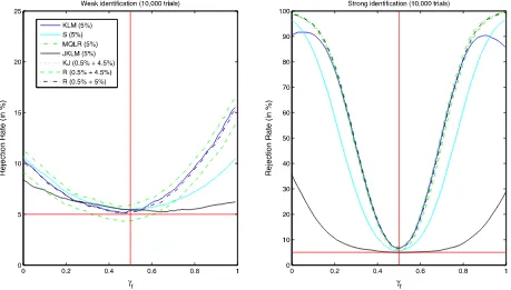
Figure 1. Power curves of 5% level tests forH0:γf =0.5 againstH1:γf =0.5. The sample size is 1,000 and the number of Monte Carlo simulations is 10,000.
of Washington Center for Statistics in the Social Sciences Seed Grant.
ADDITIONAL REFERENCES
Berger, R. L., and Boos, D. D. (1994), “P Values Maximized Over a Confi-dence Set for the Nuisance Parameter,”Journal of the American Statistical Association, 89, 1012–1016.
Chaudhuri, S. (2008), “Projection-Type Score Tests for Subsets of Parameters,” Ph.D. thesis, University of Washington, Dept. of Economics.
Chaudhuri, S., and Zivot, E. (2008), “A New Method of Projection-Based Infer-ence in GMM With Weakly Indentified Nuisance Parameters,” unpublished manuscript, University of North Carolina, Dept. of Economics.
Chaudhuri, S., Richardson, T. S., Robins, J., and Zivot, E. (2007), “A New Projection-Type Split-Sample Score Test in Linear Instrumental Variables Regression,” unpublished manuscript, University of Washington, Dept. of Economics.
Dufour, J. M. (1990), “Exact Tests and Confidence Sets in Linear Regressions With Autocorrelated Errors,”Econometrica, 58, 475–494.
Kleibergen, F., and Mavroeidis, S. (2009), “Weak Instrument Robust Tests in GMM and the New Keynesian Phillips Curve,”Journal of Business & Eco-nomic Statistics, 27, 293–311.
Silvapulle, M. J. (1996), “A Test in the Presence of Nuisance Parameters,” Jour-nal of the American Statistical Association, 91, 1690–1693.
van der Vaart, A. W. (1998),Asymptotic Statistics, Cambridge, U.K.: Cam-bridge University Press.
Rejoinder
Frank K
LEIBERGENand Sophocles M
AVROEIDISDepartment of Economics, Brown University, 64 Waterman Street, Providence, RI 02912
(Frank_Kleibergen@brown.edu;Sophocles_Mavroeidis@brown.edu)
1. INTRODUCTION
We would like to thank Fabio Canova, Saraswata Chaud-huri, John Chao, Jean-Marie Dufour, Anna Mikusheva, Norman Swanson, Jonathan Wright, Moto Yogo, and Eric Zivot for their stimulating discussions of our article. We especially like the di-versity of the different discussions, which caused them to have hardly any overlap while all of them provide insightful com-ments from the discussant’s own research perspective. Because of the small overlap of the different discussions, we comment on them separately and do so in alphabetical order.
2. CANOVA
In his discussion, Canova brings up the issue of the struc-tural versus semistrucstruc-tural specifications of the model. Indeed, we received similar comments when we presented the article at the Joint Statistical Meetings (JSM) conference in Denver, so we revised the article somewhat to give results for a particu-lar structural specification proposed by Galí and Gertler (1999).
© 2009American Statistical Association Journal of Business & Economic Statistics
July 2009, Vol. 27, No. 3 DOI:10.1198/jbes.2009.08350
332 Journal of Business & Economic Statistics, July 2009
Canova points out that not all of the parameters are identifiable in this structural specification, and this can only be achieved by a system approach. Since we did not discuss this, Canova’s discussion complements our article in an important way.
3. CHAO AND SWANSON
In their discussion of our article Chao and Swanson make two points. First, they argue that the new Keynesian Phillips curve (NKPC) might not be weakly identified. Then, partly on the basis of their first argument, they advocate the use of many instrument robust procedures for inference on the parameters of the NKPC. These two arguments are related because the many instrument robust methods require that the parameters are well identified. We discuss these two arguments in turn.
3.1 Is the NKPC Weakly Identified?
In our article, we explain that the coefficients of the NKPC are not identified when λ=0. For analytical tractability, our identification analysis was based on the pure forward-looking version of the NKPC but the result also applies to the hybrid version [γb=0 in Equation (2) in the article]; see, for example, Mavroeidis (2006). Chao and Swanson show that when the re-strictionγf+γb=1 is imposed so that the number of unknown parameters is reduced by one, the conditionλ=0 is no longer necessary for identification provided thatγf >1/2.This result was also shown inMavroeidis(2002, section 4.2), who, in ad-dition, showed that the restricted hybrid model is unidentified when λ=0 andγf ≤1/2.Furthermore, ifxt is not Granger-caused byπtin the example of Chao and Swanson, as seems to be the case with U.S. data, it can be shown that the restricted hy-brid model is unidentified whenγf≤1/2 for any value ofλ,see Mavroeidis(2002, section 4.2). However, since one of the sub-set 95% confidence intervals that we report hasγf >1/2,Chao and Swanson argue that whether the NKPC is weakly identified or not needs further examination. Incidentally, note that in the example of Chao and Swanson, whereπt Granger-causesxt,it is not clear that the model will be identified for all γf >1/2 whenλ=0.
We want to emphasize that our conclusion that the NKPC is weakly identified is based on the size of the identification ro-bust confidence sets of the parameters. It does not stem from any a priori identification analysis or from the estimates ofλ. Since the confidence sets for the semistructural parameters λ andγf reported in Figure 6 are bounded, our empirical results show that the model is not completely unidentified. The con-fidence sets for the structural parametersαandωreported in Figure 7 are, however, completely uninformative about the de-gree of backward-looking behavior,ω. They are partly infor-mative aboutα.Sinceα=1 is in the 90% confidence set, the 90% confidence set for the average duration over which prices remain fixed, which is measured by(1−α)−1,is unbounded. We believe that these results are sufficient to conclude that the NKPC is weakly identified.
Chao and Swanson argue that it is useful to have a measure of identification to assess the reliability of the point estimates of the parameters. The identification-robust confidence sets, how-ever, already provide such a measure of identification. In case
of unbounded confidence sets, the model is unidentified and we show that this result cannot be attributed to a lack of power of these identification-robust procedures relative to nonrobust methods. Moreover, Equation (26) in the article shows that the S-statistic, which is the generalization of the Anderson–Rubin (AR) statistic to the generalized method of moments (GMM), resembles a test for the rank of the Jacobian at distant values of the parameter of interest. Since the parameters are identified when the Jacobian has a full rank value, this shows that bounded S-based confidence sets provide evidence that the model is not completely unidentified. Hence, statistical inference can be conducted directly and there is no need for pretesting, even if such pretesting were possible (which is currently not the case for models like the NKPC).
The a priori identification analysis we conducted in our ar-ticle intended to highlight the dependence of the strength of identification on the value of the structural parameters in the NKPC. The strength of identification in the linear instrumen-tal variables regression model is measured by the concentration parameter and does not depend on the structural parameters. We construct the concentration parameter for the NKPC and show that it depends in a complicated way on the structural parame-ters. This dependence makes it difficult to extend methods that have been proposed to gauge the strength of the instruments in the linear instrumental variable regression model (e.g., Stock and Yogo2003and Hansen, Hausman, and Newey2008) to the NKPC.
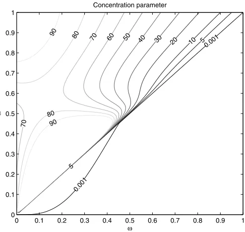
Finally, we numerically evaluate the concentration parame-ter for the restricted hybrid NKPC model over the admissible range of the structural parametersα, ω∈ [0,1]. Recall that, un-der the restrictionβ=1,Equations (33) and (34) in our article become:γf =α/(α+ω)andλ=(1−ω)(1−α)2/(α+ω). Figure 1 reports the contours of the concentration parameter
Figure 1. Approximate contours of the concentration parameter in structural NKPC withβ=1, conditional onxt∼AR(2). Reduced form coefficients and error variances are estimated using U.S. data over our estimation sample. The sample size for the concentration parame-ter is assumed to be 100.
whenxtfollows an autoregressive model of order 2 and all nui-sance parameters are calibrated to U.S. data. Upon comparison with the 90% confidence sets reported in Figure 7 of our arti-cle, we see that values of the concentration parameter of 10−3 lie within the 90% confidence set. Hence, we cannot rule out that weak identification is of empirical relevance even in the example discussed by Chao and Swanson.
3.2 Many Instruments
Chao and Swanson observe that in the NKPC and most macro models the unconditional moments from which the pa-rameters are estimated result from conditional moment restric-tions. This typically implies a large number of candidate instru-mental variables. Therefore, they argue that methods derived in the so-called many instrument literature could be relevant for the NKPC.
We agree that if one is willing to use more than a handful of instruments, it is important to use methods that are more robust to the number of instruments than the conventional two-step GMM procedure. The subset Kleibergen Lagrange multiplier (KLM) and MQLR statistics that we use in our empirical analy-sis are examples of such procedures. However, there are a few reasons that make us rather cautious in recommending the use of many moment conditions for estimating the NKPC and other related macro models.
First, it is well known that the many instrument robust proce-dures referred to by Chao and Swanson are not robust to weak identification. Our previous discussion therefore demonstrates that we do not have sufficient evidence to argue that the NKPC is sufficiently well identified for these many instrument robust methods to perform adequately.
Second, in forward-looking models the relevance of an in-strument is directly linked to its predictive content for the future value of the endogenous regressor. In the case of the NKPC, in-struments carry incremental information insofar as they help to predict future inflation beyond the first few lags of inflation and the labor share. However, there is a large literature documenting that it is rather hard to beat random walk forecasts of inflation; see Stock and Watson (2008), which leads to a relatively small number of relevant instruments.
Third, another important reason to use a limited number of instruments, which is not related to the issue of identification, is the estimation of the long-run variance of the moments. It is well known that nonparametric spectral density estimators of the long-run variance of dependent variables, such as the Newey–West estimator (see Newey and West 1987), cause sig-nificant size distortions to GMM tests; see, for example, Sun, Phillips, and Jin (2008). Neither the identification robust nor the many instrument robust procedures are immune to this problem. We have conducted several simulations of the size of GMM tests, including the ones we recommend, with different HAC es-timators and found that the size can increase dramatically with the number of instruments.
For the aforementioned reasons and since the KLM and MQLR statistics are as robust to many instrument sequences as the many instrument robust statistics and are also robust to weak identification of the parameters, unlike the many instrument ro-bust statistics, we believe they are preferable for inference on the NKPC.
4. DUFOUR
Dufour’s discussion primarily focuses on the effect of so-called missing instruments on the limiting distributions of the KLM and MQLR statistics. We therefore first address the ef-fect of missing instruments and then proceed with some further discussion of projection-based testing.
4.1 Missing Instruments
Dufour refers to the simulation study conducted by Dufour and Taamouti (2007), which shows the sensitivity of the lim-iting distributions of the KLM and MQLR statistics to miss-ing instruments. The simulation results reported in Table 1 of Dufour’s comment are striking, but the sensitivity to “miss-ing instruments” mentioned by Dufour does not result from the omission of relevant instruments. It results from their peculiar specification of the data generating process, which has the miss-ing instruments orthogonalin sampleto the included ones. This means that the missing instruments are not independent of the included instruments, and they depend on each other in a way that is unlikely to occur in practice. We show that if the missing instruments are not orthogonal to the included instruments that the size distortions of the KLM test reduce to the problem of many included instruments as discussed in Bekker and Kleiber-gen (2003).
To proceed, we first state the data generating process used in the simulation study by Dufour and Taamouti (2007), which is identical to the one in Dufour’s comment. We then show that the size distortions result from the orthogonality of the miss-ing instruments to the included ones. We explain that this size distortion arises mainly from the estimation of the covariance of the errors, which is used in the computation of the KLM and MQLR statistics; see Kleibergen (2002). Since these covariance estimators are not needed for the AR statistic, its distribution is not affected by the missing instruments under the null. How-ever, we show that this orthogonality assumption adversely af-fects the power of the AR statistic, which becomes biased, and has a similar effect on the first-stageF-statistic for the coeffi-cients of the included instruments.
The simulation study of Dufour and Taamouti (2007) uses the model
y1=Y1β1+Y2β2+u,
(1) (Y1...Y2)=X22+X3δ+(V1...V2),
withy1,Y1,Y2,X3:T×1,X2:T×k2,and
vec(ut...V1t...V2t) iid
∼N(0, ),
(2)
=
1 0.8 0.8
0.8 1 0.3 0.8 0.3 1
.
TheT×k2matrixX2contains the included instruments while
the T×1 vector X3 is a vector of omitted instruments.
Du-four and Taamouti (2007) specify the vector of missing instru-ments such that it is orthogonal to X3, X3′X2≡0. They
sim-ulate the elements of X2 and X3 as iid N(0,1)random
vari-ables and orthogonalize X3 with respect to X2. Dufour and
334 Journal of Business & Economic Statistics, July 2009
Taamouti (2007) keep the instruments fixed in repeated sam-ples, but this is inessential for the results. In his discussion, Dufour uses random instruments, so we do the same in our simulations here. The results are qualitatively the same with fixedX.Dufour and Taamouti (2007) set the parameter values atβ1=12, β2=1,andδ=λ(1...1). Their parameter matrix2
is such that2=ρ/√T, whereρis 0.01 or 1,with the
ele-ments on the main diagonal of thek2×2 matrixequal to one
and the remaining off-diagonal elements are all equal to zero. This implies that the concentration matrices, which are equal to′2X2X22,are roughly equal to which shows that the included instruments are basically weak (ρ=1)or irrelevant (ρ=0.01). The sample sizeT is equal to 100 and the number of instruments k2 varies between 2
and 40.
To show the implications of the orthogonality ofX2andX3,
we consider the score vector with respect to(β1, β2)of the
lin-ear instrumental variables regression model at the true value of β1andβ2, which is proportional to (see Kleibergen 2002):
u′Z˜2(β1, β2)=u′PX2(Y1
tic is a quadratic form of the score vector in (3). Hence, any peculiar behavior of the KLM statistic is directly related to the score vector. If X2 andX3 are orthogonal, soPX2X3=0,the
score vector in (3) simplifies to
u′Z′˜2(β1, β2)=u′PX22+u′PX2(V1
It is important to note that except for the last element of the above expression, the missing instruments have dropped out of all the other elements.
WhenX3 is missing, it becomes part of the residual in the
first-stage regression, and the key idea behind the score vector is to orthogonalize the first-stage residual with respect to the structural erroru. Now, whenuandX3are independent in the
population, there is always some nonzero sample correlation between u andX3. The expression of the score vector in (4)
shows that the orthogonality ofX2andX3prevents the sample
correlation betweenuandX3from affecting the first element of
the score vector. The sample correlation betweenuandX3still
affects the second part of the score vector. Hence, because of the orthogonality ofX2andX3,uand[(Y1...Y2)−uσσˆˆuV
uu]exhibit sample correlation although they are uncorrelated in the popu-lation. One can therefore obtain any kind of size distortion by appropriately specifyingδorλ.
Another consequence of the orthogonality of X2 andX3 is
that the AR test is not unbiased because its power can be lower than the level of the test under the alternative, and when the included instruments are sufficiently weak, the power of the AR test is actually maximized under the null. To see this, note that the specification of the AR statistic that tests H0:β =
(β1,0, β2,0)′when the true value isβ=(β1, β2)′reads
where we used the fact that
y1−(Y1...Y2)
and that, because of the orthogonality ofX2andX3,X3drops
out of the numerator. Whenδ is different from zero, the esti-mate of the variance in the denominator is inflated, and this un-ambiguously reduces power. In the limiting case with2=0,
the power of the AR test is equal to its level whenδ=0,and it must therefore be less than the level forδ >0.This is shown in the simulations reported below based on Dufour’s example where the included instruments are very weak. This also im-plies that for a given nonzero value ofδthe rejection frequency of the AR statistic is maximized at the true value ofβ.Hence, the orthogonality ofX2andX3leads to a biased AR test, which
leads to the strange outcome that the true value is the most ob-jectionable value.
The odd behavior of the AR statistic whenX2andX3are
or-thogonal extends to similar nonstandard behavior of other sta-tistics, such as the first-stage Wald statistic that tests whether 2is equal to its true value. Because the covariance matrix
es-timator is the only element of this Wald statistic that depends onδ, it overstates the variance so the Wald test will be under-sized.
The above shows that the orthogonality of the missing instru-mentX3compared to the included instrumentX2 explains the
strange behavior of the different statistics, including the AR sta-tistic, whose power function is maximized under the null when identification is weak. IfX2andX3are not orthogonal, the effect
of missing instruments on the limiting distributions of the KLM and MQLR statistics is identical to the effect of many instru-ments on the limiting distribution of the KLM statistic, which is discussed in Bekker and Kleibergen (2003). This is because missing relevant instruments essentially blow up the variance of the error term in the first-stage regression and therefore reduce the concentration parameter. When the number of included in-struments is also large, this leads to the many weak inin-struments problem discussed in Bekker and Kleibergen (2003).
To show this, we consider the estimator of2,˜2(β1, β2),
the true values of the covariance parametersσuVandσuu, there is no sensitivity to missing instruments. Thus the sensitivity to missing instruments results from the last part of the expression in (7). We therefore analyze the behavior of the covariance es-timatorσˆuV:
The convergence rates ofψuV andψuX3 in the expression for
ˆ
where ψuV and ψuX3 are independently normally distributed
with mean zero.
The expression of the covariance estimator in (8) shows that the sensitivity to missing instruments results from the higher-order elements, √1
T−k2ψuVand
1 √
T−k2ψuX3δ.The convergence
rate of these elements depends on the number of instruments. Bekker and Kleibergen (2003) show that the limiting distrib-ution of the KLM statistic when the number of instruments is proportional to the sample size is bounded between a χ2(m) and a χ12−(mα) distribution withmthe number of structural para-meters andα=limk2,T→∞
k2
T. Theχ
2(m)lower bound is
at-tained when the structural parameters are well identified and the χ12−(mα) upper bound is attained when the structural parame-ters are completely unidentified.
To illustrate the above remarks, we revisit the simulation ex-ercise of Dufour and Taamouti (2007). Table1shows the rejec-tion frequencies of the KLM test using the same data generat-ing process as in Dufour’s comment. We only show the results for the KLM statistic since the results for the MQLR statistic are similar. Table1 shows rejection frequencies for the KLM test under four different scenarios. The first scenario, listed as “Orth,” matches the results reported in Dufour’s Table 1 under the heading “K” and has the missing instrument orthogonal to the included ones. The second scenario, listed as “Known cov,” uses the true values of the covariance parametersσuV andσuu in the computation of the KLM statistic. The third scenario, listed as “Nonorth,” does not force the missing instrument to be orthogonal to the included ones. The fourth scenario, listed as “Upper,” uses nonorthogonal missing instruments and critical values from the χ12−(2α) upper bound on the limiting distribution obtained by Bekker and Kleibergen (2003).
It is clear from the results that the large size distortions occur only in the case of orthogonalized missing instruments, and the size distortions get larger as the relevance of the missing instru-ment increases (the caseλ=10 means that the concentration parameter associated with the missing instrument is 20,000). Table1shows that there is no size distortion when we use the known values of the covariance parametersσuVandσuu, in ac-cordance with our above discussion. When we use missing in-struments that are not orthogonal to the included ones, Table1 shows that the size distortions do not depend on λ (i.e., the strength of the missing instruments) and only depend on the number of included instruments k2. This confirms our
previ-ous analysis, which showed that the effect of missing instru-ments on the limiting distribution results basically from the use of many instruments. This is further confirmed when we use critical values that result from the upper bound on the limiting distribution obtained by Bekker and Kleibergen (2003). Since the included instruments are very weak, the limiting distribu-tion of the KLM statistic coincides with the upper bound, which is confirmed by the rejection frequencies that coincide with the size of the test.
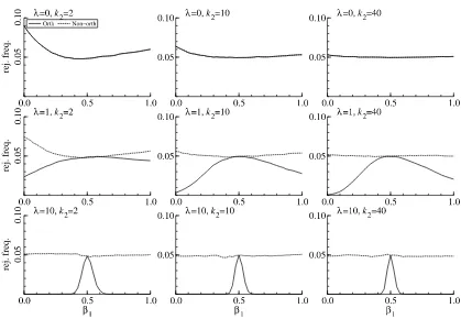
Next, we turn to our remarks concerning the effect of or-thogonal missing instruments on the power of the AR statistic. Figure 2 shows the power of the AR statistic in (5) for test-ingH0:β1=12, β2=1 for different values ofβ1 whileβ2 is
fixed at its true value (when we varyβ2,the results are
qualita-tively the same). The power curves in Figure2result from the data generating process used by Dufour and Taamouti (2007) withX2orthogonal toX3,which is indicated by “Orth,” and the
336 Journal of Business & Economic Statistics, July 2009
Table 1. Rejection frequencies of KLM statistic in case of missing instruments
k2 Orth Known cov Nonorth Upper Orth Known cov Nonorth Upper
λ=0 andρ=0.01 λ=0 andρ=1
2 5.18 4.87 5.18 4.85 5.18 4.87 5.18 4.85
3 5.52 4.94 5.52 5.03 5.53 5.3 5.53 5.14
4 5.54 4.88 5.54 4.93 5.46 5 5.46 4.8
5 5.93 5.13 5.93 5.23 5.78 4.88 5.78 5.04
10 7.3 5.17 7.3 5.52 6.4 5.06 6.4 4.76
20 9.45 4.97 9.45 5.4 7.82 4.83 7.82 4.11
40 17.03 4.87 17.03 5.58 13.55 5.08 13.55 3.93
λ=1 andρ=0.01 λ=1 andρ=1
2 5.18 4.87 5.18 4.85 5.18 4.87 5.18 4.85
3 7.7 4.94 5.58 5.23 5.78 5.3 5.7 5.26
4 11.07 4.88 5.82 5.25 6.26 5 5.95 5.25
5 14.8 5.13 6.31 5.43 7.12 4.88 6.37 5.52
10 33.32 5.17 7.35 5.55 14.94 5.06 7.33 5.36
20 59.28 4.97 9.62 5.61 37.89 4.83 9.43 5.35
40 78.04 4.87 16.83 5.45 68.23 5.08 16.63 5.22
λ=10 andρ=0.01 λ=10 andρ=1
2 5.18 4.87 5.18 4.85 5.18 4.87 5.18 4.85
3 11.26 4.94 5.52 5.15 9.34 5.3 5.6 5.23
4 19.34 4.88 5.84 5.24 15.36 5 6.07 5.47
5 28.82 5.13 6.27 5.44 22.79 4.88 6.26 5.42
10 73.36 5.17 7.42 5.56 63.09 5.06 7.41 5.33
20 95.16 4.97 9.65 5.57 91.22 4.83 9.64 5.33
40 97.82 4.87 16.92 5.51 96.68 5.08 16.63 5.4
NOTE: Orth: orthogonal instruments. Known cov: known covariance. Nonorth: nonorthogonal instruments. Upper: critical values result from the upper bound on the limiting distribu-tion.
Figure 2. Power of the AR statistic for testingH0:β1=0.5, β2=1 for different values ofβ1andβ2equal to 1. Orth: orthogonal instruments. Nonorth: nonorthogonal instruments.
same data generating process withX2not orthogonal toX3,
in-dicated by “Nonorth.” The power curves in Figure2that result from the orthogonal and nonorthogonal specification are iden-tical whenλ=0, which is the case of no missing instrument. Whenλ=1 or 10,the power of the AR statistic is minimized at the true value in case of nonorthogonal instruments while it is maximized at the true value in case of orthogonal instruments. Figure2 therefore shows that the odd behavior of the power curve of the AR statistic results from the orthogonality ofX2
andX3and not from the property thatX3is a missing
instru-ment.
Table1, Figure2, and our previous discussion show that the size distortions reported by Dufour and the peculiar behavior of the AR statistic with respect to its power result from the orthogonality of the missing instrument compared to the in-cluded ones. When the missing instruments are not orthogonal: (i) the effect of the missing instruments on the limiting distri-bution results from the sensitivity of the limiting distridistri-bution to many instruments and (ii) the AR test is unbiased. Instru-ments that are orthogonal to one another are not independently distributed. This is the reason for the peculiar behavior of the different statistics, and it makes the relevance of the simulation study of Dufour and Taamouti (2007) somewhat questionable for practical purposes. In fact, if one insists on the principle of robustness against such a type of missing variables, it is easy to construct examples in which no statistic (including the AR statistic) has correct size. Specifically, such an example can be constructed by considering the case of an exogenous variable X3that has been omitted from the structural equation, that is, y=Y1β1+Y2β2+X3δ+u. In applied work researchers rarely
observe all the relevant measurable characteristics that may af-fect a particular outcome of interest, and these omitted vari-ables form part of the error term. If the unobserved characteris-ticX3is uncorrelated with the included instruments,X2,valid
inference can be drawn forβ1andβ2.However, if the omitted
variable is orthogonal toX2,then even the AR statistic will be
severely size distorted. We think that this situation is as unreal-istic as missing instruments in the first-stage regression that are orthogonal to the included ones.
4.2 Projection Methods
For the same statistic of interest, the subset versions that we use dominate their projection-based counterparts with respect to power and also show that the projection-based statistics are conservative. Dufour advocates the use of projection-based sta-tistics and puts forward three arguments:
1. Use of the subset statistics relies on an asymptotic argu-ment. We agree that one has to be careful with applying asymptotic arguments. The research on weak instrument robust statistics is largely motivated by the bad perfor-mance of such asymptotic arguments with respect to the traditionally used statistics. The reason why these asymp-totic arguments do not perform very well is, however, the high-level assumption with respect to the rank of the Ja-cobian and not the inappropriateness of asymptotic argu-ments in general. For example, central limit theorems hold
under mild conditions (see, e.g., White 1984) and pro-vide the foundation for statistical inference in most econo-metric models. The limiting distributions of the weak in-strument robust statistics only require such a central limit theorem to hold (see Assumption 1) and therefore apply quite generally. Use of such central limit theorems leads to more robust statistical inference than the one which re-sults from assuming a specific distribution for the data and which would lead to so-called exact inference.
2. The regularity conditions for the derivative in GMM puts restrictions on the model. We agree that making assump-tions about the derivative puts some restricassump-tions on the model compared to only using the moments themselves. As usual, imposing more structure on the model trades off robustness for power. Arguably, there are cases in which the additional restrictions imposed by our assump-tion on the derivative area prioriquestionable (e.g., the example studied in Mavroeidis, Chevillon, and Massmann 2008, which uses projection-based tests only). However, we think that for the application that we looked at, this assumption is mild. See also our response to Mikusheva’s comment below.
3. The limiting distributions of subset statistics are sensitive to missing instruments. We have extensively addressed this point above.
5. MIKUSHEVA
Mikusheva raises two concerns about the relevance of As-sumption 1 for the NKPC. AsAs-sumption 1 states that the moment conditions¯ft(θ )and their Jacobianq¯t(θ )are approximately nor-mally distributed. Mikusheva argues that the normal approxi-mation might be inaccurate because of (i) the high persistence in inflation and (ii) the large dimension ofq¯t(θ )relative to the sample size. We discuss each of these arguments consecutively. We agree with Mikusheva that persistence in inflation can in-validate Assumption 1. To address this issue, in our empirical analysis we used the lags ofπ instead ofπ as instruments. Mikusheva rightly observes that this is sufficient to ensure the approximate normality of the moment conditions under the null ft(θ0), which will contain terms of the formπt−iet,whereet is MA(1), but not necessarily under the alternative, in general. This is because under the alternative,ft(θ )also contains terms of the form πt−i(γf −γf,0)πt+1 andπt−i(γb−γb,0)πt−1,
which will not be approximately normal whenπtis nearly inte-grated.
However, there are special cases in which Assumption 1 can be verified, and our empirical application with the restriction γf +γb=1 is such a special case. This is because the restric-tionγf +γb=1 makes the model linear in2πt+1[see
Equa-tion (32) in the article], and the moment condiEqua-tions become Zt(πt−γf2πt+1−λxt).As a result, neither the moment con-ditions under the alternative, nor their Jacobian involve any lev-els of the potentially integrated seriesπt, and our Assumption 1 can be verified. This argument does not apply more generally to the unrestricted specification. Indeed, this is precisely the reason why in a related article studying the NKPC with learn-ing, Mavroeidis, Chevillon, and Massmann (2008) use only the S-statistic for the full parameter vector, for which the relevant
338 Journal of Business & Economic Statistics, July 2009
part of Assumption 1 can be verified under the null hypothe-sis. Nonetheless, in view of similar results in the cointegration literature, where the estimators of the parameters of the cointe-grating vector have normal limiting distributions, it is possible that we might have (mixed) asymptotic normality of the score vector while the derivatives of the moments do not converge to a normal distribution. Even though we did not need to investi-gate this further for our application, we believe that this issue is of considerable general interest and deserves further study.
Mikusheva’s second point concerns the dimensionality of the moment and derivative vector that is involved in Assumption 1. We agree that the dimensionality of the moment and derivative vector is quite large. Although the limiting distributions of the identification robust KLM and MQLR subset statistics do not alter under a many instrument limit sequence, the dimension-ality is an issue especially with respect to the involved HAC covariance matrix estimators. We have conducted several sim-ulations of the size of GMM tests, including the ones we rec-ommend, with different HAC covariance matrix estimators and found that the size can increase dramatically with the number of instruments. Our main concern with respect to the dimension-ality is therefore not so much the appropriateness of the central limit theorem but more so the convergence of the HAC covari-ance matrix estimators.
6. WRIGHT
One of the main points of Wright’s discussion is that the quest for strong instruments in the NKPC is essentially the same problem as the search for good forecasts of inflation and mea-sures of economic slack. It is well known that pooling forecasts typically reduces the mean square prediction error especially when the pooled forecasts are not highly correlated. Wright therefore proposes to use the Greenbook and professional fore-casts as additional instruments. These forefore-casts are judgmental, and therefore not highly correlated with the forecasts that result from autoregressions, which are implicitly used in the GMM estimation procedure. Since the Greenbook forecast is known to improve model-based inflation forecasts, one might expect that it can also improve the identification of the parameters in the NKPC. Figure 1 in Wright’s discussion provides evidence of this as it shows that the S-based confidence set of (λ, γf) reduces considerably when we use the Greenbook forecast as an additional instrument. It is interesting to extend this analy-sis further and incorporate more powerful identification robust statistics like the KLM and MQLR statistics.
The second point in Wright’s discussion concerns a differ-ent model of the NKPC that allows for exogenous time-varying drift in inflation. Cogley and Sbordone (2008) develop such a model and show that its coefficients are time-varying even though the underlying structural parameters, such as the de-gree of price stickiness, are constant. Since this model is sub-ject to the same possible identification problems, we agree with Wright that it is important to apply identification robust meth-ods for inference in this model, too. The main challenge is not that the Cogley and Sbordone (2008) model has more parame-ters than the standard NKPC, but rather that its coefficients are time-varying. This makes it hard to apply GMM methods di-rectly. Moreover, as Wright points out, nonstationarity in infla-tion complicates the asymptotic distribuinfla-tion of the identificainfla-tion
robust tests. This is similar to the point made by Mikusheva, which we managed to address in the restricted version of the standard NKPC by using lagged changes in inflation as instru-ments. However, this trick may not work more generally, so this remains an important open issue for future research.
Finally, Wright argues that it would be useful to have a mea-sure of the strength of identification as a way to assess the reli-ability of point estimators and standard errors. A similar com-ment was made by Chao and Swanson. As we already stressed earlier, the identification robust confidence sets provide such a measure of identification. If they are tightly concentrated around the CUE, then the point estimates are reliable, other-wise they are not. Moreover, the fact that the identification ro-bust confidence sets are computationally more demanding than the usual standard error bands should not be used as an argu-ment against their use, since efficient computer programs are readily available. Judging from recent developments in empir-ical macroeconomics, it seems that leading researchers are not averse to using methods that are even more computationally de-manding than the ones we propose.
7. YOGO
Yogo discusses our empirical findings on the NKPC from the perspective of the results documented in the literature. He shows that the 95% confidence sets on the slope coefficient and forward-looking parameter encompass those stated in Galí and Gertler (1999) for both of their normalizations. He states that this is indicative of the weak identification of these parameters with which we clearly concur.
An interesting perspective that Yogo takes from the large confidence sets of the structural price adjusment and backward-looking parameters is that it might be useful to incorporate in-formation from microdata. Yogo shows that usage of a plug-in microdata estimate of the price adjustment parameter reduces the 95% confidence set for the slope and structural backward-looking parameter but not of the forward-backward-looking parameter. This result is of considerable interest and shows a way of proving the precision of the empirical analysis that we find im-portant.
8. ZIVOT AND CHAUDHURI
Zivot and Chaudhuri focus their discussion on the implemen-tation and performance of the Robins test. Figure 3 of our article shows the power curves of the subsetS-statistic and projection and Robins tests that are based on theS-statistic. Figure 3 shows that the projection and Robins tests are conservative and have less power than the subsetS-statistic.
Our implementation of the Robins test is geared towards the subsetS-statistic in the sense that the test attempts to reduce the power loss of the projection-basedS-statistic relative to the sub-setS-statistic. Zivot and Chaudhuri show that our version of the Robins test can be improved upon by gearing the Robins test to-wards the KLM statistic. In case of two parameters(α, β),the Robins test for testingH0:β=β0would then consist of
con-structing a(1−ν)×100% confidence set forαusingS(α, β0)
and then, for each value ofαinside the(1−ν)×100% con-fidence set, testing the hypothesis H0:β =β0 using a
condi-tional KLM statistic forβ,which they define in their discus-sion and also in Chaudhuri (2007) and Chaudhuri et al. (2007). The power curves reported by Chaudhuri and Zivot in Fig-ure 1 of their discussion result from this implementation of the Robins test and are similar to the ones we reported in Figure 3 of our article except that now the power curve of the Robins test is to be compared with the power curve of the KLM–JKLM combination and the MQLR statistic, which are the most pow-erful subset statistics. This is an interesting result since it shows that, although the Robins test remains conservative, it can be constructed in a way that is geared towards the most powerful statistic and can be made almost as powerful. This approach therefore offers a general principle for preserving the size of tests on subsets of the parameter with good power properties.
The manner in which the Robins test advocated by Zivot and Chaudhuri operates is similar to the combination of the KLM and JKLM statistic advocated by Kleibergen (2005) to avoid spurious power declines of the KLM statistic. Some issues that are of interest to investigate further for the Robins test are: (i) its
performance at distant values of the hypothesized parameter for which the subset statistics resemble identification statistics and (ii) its ease of implementation since the construction of the (1−ν)×100% confidence set might be computationally de-manding.
ADDITIONAL REFERENCES
Bekker, P. A., and Kleibergen, F. (2003), “Finite-Sample Instrumental Variables Inference Using an Asymptotically Pivotal Statistic,”Econometric Theory, 19, 744–753.
Cogley, T., and Sbordone, A. M. (2008), “Trend Inflation and Inflation Persis-tence in the New Keynesian Phillips Curve,”American Economic Review, 98, 2101–2126.
Hansen, C., Hausman, J., and Newey, W. (2008), “Estimation With Many In-strumental Variables,”Journal of Business & Economic Statistics, 26, 398– 422.
Mavroeidis, S. (2002), “Econometric Issues in Forward-Looking Monetary Models,” Ph.D. thesis, Oxford University, Oxford.
Stock, J. H., and Yogo, M. (2003), “Testing for Weak Instruments in Linear IV Regression,” Technical Working Paper 284, National Bureau of Economic Research.
Sun, Y., Phillips, P. C. B., and Jin, S. (2008), “Optimal Bandwidth Selection in Heteroskedasticity-Autocorrelation Robust Testing,”Econometrica, 76 (1), 175–194.