CADASTRAL DATABASE POSITIONAL ACCURACY IMPROVEMENT
N. M. Hashim a*, A. H. Omar a*, S. N. M. Ramli a*, K.M. Omar a*, N. Din a, *
a
Dept. of Geomatic Engineering, University Technology Malaysia, Skudai, Johor Bahru, MALAYSIA – *[email protected], *[email protected], *[email protected],
*[email protected], *[email protected]
KEY WORDS: Positional Accuracy Improvement, Legacy Dataset; Cadastral Database Modernization
ABSTRACT:
Positional Accuracy Improvement (PAI) is the refining process of the geometry feature in a geospatial dataset to improve its actual position. This actual position relates to the absolute position in specific coordinate system and the relation to the neighborhood features. With the growth of spatial based technology especially Geographical Information System (GIS) and Global Navigation Satellite System (GNSS), the PAI campaign is inevitable especially to the legacy cadastral database. Integration of legacy dataset and higher accuracy dataset like GNSS observation is a potential solution for improving the legacy dataset. However, by merely integrating both datasets will lead to a distortion of the relative geometry. The improved dataset should be further treated to minimize inherent errors and fitting to the new accurate dataset. The main focus of this study is to describe a method of angular based Least Square Adjustment (LSA) for PAI process of legacy dataset. The existing high accuracy dataset known as National Digital Cadastral Database (NDCDB) is then used as bench mark to validate the results. It was found that the propose technique is highly possible for positional accuracy improvement of legacy spatial datasets.
* Corresponding author
1. INTRODUCTION
Many countries around the world have recognized and appreciated the value of accurate digital cadastral database. Theoretically, an accurate, efficient and updated cadastral database offers the better basis for planning and implementation of variety of real estate application (Durdin, 1993; Effenberg et al. 1999; Ting et al., 1999). The advancement in spatial based technology like Geographic Information System (GIS) also suggested an urgent need to maintain the spatial data in high accuracy to represent the real world.
Principally, numerous spatial datasets were previously digitized from hardcopy maps. The legacy datasets in use today are a combination of data from different sources, of technologies and measurement techniques. As a result, these legacy datasets have relatively low positional accuracy caused by errors resulting from the production and measurement method employed according to the technological and legal changes over time (Sisman, 2014). In addition, the common error in digitizing process such as distortion of source map, digitizing operational errors and ground coordinate system constituted a combination of systematic and random errors (Tong, Shi, & Liu, 2009). However, the urgency of updating legacy dataset is extremely crucial, the needs for combine spatial data from different sources and accuracy has dramatically increased. This process is crucial to allow different datasets to be jointly presented and analyzed. The process requires an understanding about the positional accuracies of the geometries in the datasets to avoid mismatches and misinterpretations of geospatial data.
Generally, resurvey, reprocessing the existing survey data and upgrading the existing cadastral datasets are the potential
approaches for improving the legacy cadastral datasets. Resurvey all the cadastral parcel probably is the best technique to generate the new accurate dataset, however this process require lengthy time and estimated cost is very high (Arvanitis et al., 1999). Meanwhile, Buyong et al. (1992) and Durdin (1993) suggested that maintaining the old measurement and incorporating the new measurements will suffice for upgrading legacy datasets. However, Perelmuter et al. (1992) stated that the incorporating is unsuitable due to weakness of the original control network (datum) and field book record system. Additionally, from the economic perspective, 20000 existing field books for instance, will require hundreds of operators and take many years to accomplish (Fradkin et al., 2002).
A possible alternative for improving the legacy datasets with realistic cost is transforming the legacy dataset into new system. This high possibility supported by the advancement of satellite base technology especially Global Navigation Satellite System (GNSS). Possibly, the coordinate accuracy of the legacy dataset can be highly improved. Furthermore, the availability of high resolution aerial imagery offer high possibilities of using imagery as background when underlays to spatial dataset (Hope et al., 2008). The imagery which has high quality spatial resolution and absolute accuracy like Quick Bird can be used as a base map to check the relative position of the adjusted legacy datasets.
Essentially, the legacy dataset accuracy has to be improved line with the current high accuracy spatial technology. As a result, many organizations and researchers around the world used PAI approach for upgrading legacy datasets into high accuracy dataset (Donnelly et al.2006; Fradkin et al., 2002; Hesse et al., 1990; Morgenstren, 1989; Tamim, 1995). Based on the The International Archives of the Photogrammetry, Remote Sensing and Spatial Information Sciences, Volume XLII-4/W5, 2017
importance of PAI, the focus of this paper is to propose the PAI method using angular based Least Square Adjustment (LSA). The detail discussion on PAI is explained in the following section.
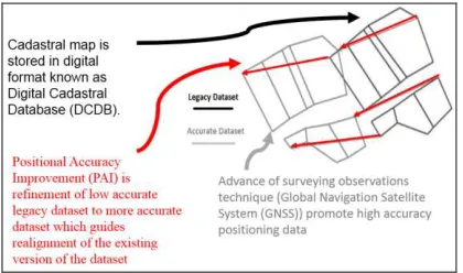
Figure 1. PAI concept (Hashim et al, 2016)
2. POSITIONAL ACCURACY IPROVEMENT
PAI is a process of improving the position of the geometric coordinates of a feature in a geospatial dataset to represent its actual position (Rönsdorf, 2008). The PAI can be classified as the improvement of low accurate legacy dataset to more accurate dataset. Figure 1 illustrates the concept of PAI (Norshahrizan et al, 2016).
PAI is commonly applied in two situations, PAI of Reference Data and PAI of User Data (Rönsdorf, 2008). The PAI of Reference Data links with improving the position of geometries in a reference dataset that describes physical or abstract features of the earth. The features position relate to the absolute position in a standard Coordinate Reference System such as Geocentric Datum of Malaysia 2000 (GDM 2000) in case of Malaysia or WGS-84 in global coordinate system. Meanwhile, the PAI of User Data describes the successive synchronization of legacy datasets with the already positionally improved reference dataset in order to retain the relationships between geometries.
To achieve an optimal solution in PAI, the method of LSA is often employed towards improving the positional accuracy of spatial datasets (Tamim 1995, Wolf and Ghilani 2006, Merritt and Masters 1999, Gielsdorf et al. 2004, Merritt 2005, Tong et al. 2005, Casado 2006, Hope et al. 2008, Tong et al. 2009). The LSA method is a well-established technique for solving an overdetermined system of equations by minimizing a weighted quadratic form of the residuals. Its application in estimating parameters in coordinate transformation can be found in literature; for example, Mikhail and Ackemann (1982), Wolf and Ghilani (2006), and Koch (1999). Tamim (1995) presented a methodology to create a digital cadastral overlay through upgrading digitized cadastral data. Merritt and Masters (1999) and Merritt (2005) developed the spatial adjustment engine based on the least squares method and applied it to improve the accuracy of cadastral data in Australia. Tong et al. (2005) presented a least squares adjustment model to resolve inconsistencies between the digitized and registered areas of cadastral parcels, and further improved the adjustment model by introducing scale parameters to reduce the influence of systematic error in the adjustment (Tong et al. 2009). Felus (2007) presented a workflow of three steps used to enhance the spatial accuracy of digital cadastral maps: a global
transformation from an old local system to a GPS-based WGS-84 system; a rubber-sheeting transformation for modifying boundary corners to fit existing ground features; and a LS adjustment with stochastic constraints to include additional cadastral information and geometric conditions. Hope et al. (2008) proposed a method of least squares with inequalities for data integration, in which topological relationships are modeled in the form of inequalities and optimal positioning solutions are obtained while preserving the spatial relationships among features.
Since the legacy dataset are less accurate in positioning, the integration of legacy datasets and highly accurate data such as those from GNSS is one of the most possible methods to improve the legacy datasets accuracy (Hope et al., 2008). However, it was found from Hope et al. (2008) that by simply replacing a sample of legacy dataset with more accurate version will lead to a distortion of the neighboring geometry (Figure 2). In addition, the relative geometry of the legacy datasets is often better than its absolute accuracy and supposed to be the spatial relationship or relative geometry between features must be preserved.
Figure 2. Cadastral boundaries (Solid Lines) and higher accuracy (Dashed Lines). Polygon xady is distorted if point
abcd are simply replaced by ABCD (Hope et al., 2008)
The previous studies discussed above largely used the additional new observations which link with the legacy data for maintaining the geometry of adjusted data. In this study, the existing data alone from certified plan is used for maintaining the geometry of legacy data in the adjustment stage. The following section describes how the distance, bearings and angles are used in the LSA process.
2.1 Least square adjustment (LSA)
LSA is a model of solution widely used in the disciplines of surveying. The conventional Bowditch method is known as an arbitrary method since the corrections to the observations are applied irrespective of their uncertainties, whereas the least square adjustment method is more advanced technique. It adjusts observations based on the laws of probability, which models the occurrence of random errors (Halim et al., 2001). In other words, the LSA principle is such that the squares of the The International Archives of the Photogrammetry, Remote Sensing and Spatial Information Sciences, Volume XLII-4/W5, 2017
residuals must be minimized. Equation (1) expresses the fundamental principle of least squares:
(1) where v= residual
There are two mathematical models in LSA, stochastic and functional model. The stochastic model involves the determination of variances and the weights of the observations. A functional model is an equation or set of equations that represents or defines an adjustment condition. There are two types of functional models, the conditional and parametric adjustments. In a conditional adjustment, geometric conditions are compulsorily imposed on the measurement and their residuals, for instance, the sum of the angles in a closed polygon is (n-2) x 180. In the parametric adjustment, observations are expressed in terms of unknown parameters that were never observed directly. For example, the well-known coordinate equations are used to model the angles, directions, and distances observed in a horizontal plane survey. The adjustment yields the most probable values for the coordinates (parameters), which in turn provide the most probable values for the adjusted observations.
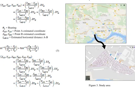
In this study, the parametric adjustment of functional model is applied. The three mathematical models of observations, horizontal angle, azimuth and distance were used in the adjustment process. The mathematical model of bearing, horizontal angle and distance observation are like equations (2), (3) and (4) respectively (Amat, 2007; Setan, 1995; Wolf and Ghilani (2006).
(2)
where = Bearing
= Point A estimated coordinate = Point B estimated coordinate = Estimated horizontal distance A-B
(3)
where = Horizontal angle
= Point A estimated coordinate = Point B estimated coordinate = Point D estimated coordinate = Estimated horizontal distance A-B = Estimated horizontal distance A-D
(4)
where = Distance
= Point A estimated coordinate = Point B estimated coordinate = Estimated horizontal distance A-B
3. METHODOLOGY
The research study area is in Kampung Pasir, Mukim Pulai, Johor Bahru District as shown in Figure 3. The area covers 77 parcels and the details of the data sources are illustrated in Table 1. The raw data for adjustment process was acquired from DSSM Johor in the form of Digital Cadastral Data Base (DCDB) or commonly known as Pangkalan Data Ukur Kadaster (PDUK). In this paper, the existing technique applied by DSMM is declared as DSMM Technique. Meanwhile, the proposed technique to produce the new accurate dataset is known as PAI Technique.
Figure 3. Study area
Table 1. Data sources
Location Kampung Pasir, Mukim Pulai, Daerah Johor Bahru, Johor, Malaysia
Parcel number 4169-4189, 4199-4225, 119251- 119277 & 119279
Certified Plan (CP) CP 40225 and CP 120293
Data PDUK (Block boundary line, CRM, Lot) Data form Bearing and distance
Data format .tab
Adjustment
Software Star*net
Figure 4. Interior angle extraction
The first step involves the calculation of interior angle of cadastral parcel. The existing raw data in LSA applied by DSMM are bearing and distance. The proposed method in this study is based on the angular and distance based LSA. The main justification of using angle method is to extract the independence or direct observation of raw data which contained minimum gross and systematic error. The bearing value is a very dependent data where it is largely based on the sources of the initial bearing. The common practice of the DSMM in the previous work is based on the solar observation and interior angle of three good boundary marks. As a result, it is extremely difficult to verify the quality of the reference bearing used in the previous work. In this study, the interior angle of these data is considered as an independent data which is calculated from the bearings of two boundary lines. Although the bearing control contains gross and systematic error, the interior angle between two boundary lines is free from the both factors.
The Star*net software has been used for the adjustment purposes. The Star*net is a rigorous least squares analysis software designed to adjust 2D and 3D survey networks. The output consists of a file of adjusted station coordinates and a statistical analysis of the adjustment. In addition, the graphical facilities are provided to allow the user to plot the network, including error ellipses of the adjusted points and relative error ellipses between stations. Star*net has the capacity to weight all input data both independently and by category which means that data can be defined as being FREE or FIXED and anything in between. The Star*net has the ability to control the weighting of input data where Giving accurately known measurements more weight than those measurements known to be less accurate.
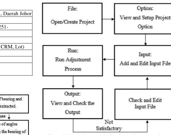
The detail step of the processing in Star*net is shown in Figure 5. A new project is created which have two input file, bearing-distance and angle-bearing-distance. The bearing-bearing-distance input data is the current technique used by DSMM, meanwhile, the angle-distance input data is the new approach which is proposed in this study.
Figure 5. Processing stage in Star*net adjustment software
The final output of the adjustment in Star*net is the adjusted coordinate of entire boundary marks. The final coordinate will be exported to the dxf, coverage and shapefile format for further graphic and spatial based analysis. The AUTOCAD and ARCGIS software are the main tools for the processing. The final output of this process will be submitted in the accurate cadastral database. Figure 6 describes the entire process of suggested PAI as discussed above.
Figure 6. Accurate cadastral database development
4. RESULT AND ANALYSIS
In the verification stages, the output of the PAI Technique was compared to the result of DSMM Technique. The verification is based on four factors, area, bearing, distance and coordinate.
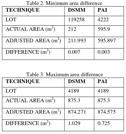
Table 2, 3, and 4 show the sample results of area comparisons by DSMM and PAI techniques. The actual area represents the area extracted from original certified plan (CP) and the adjusted area is obtained from the two different techniques. The results shown are selected from the minimum and maximum area differences of both methods.
Based on the DSMM Technique, the larger area differences given is 1.209 m2 while the larger value given by PAI Technique is 0.725 m2. In the meantime, the smallest The International Archives of the Photogrammetry, Remote Sensing and Spatial Information Sciences, Volume XLII-4/W5, 2017
differences of both techniques are 0.007 m2 and 0.003 m2
In the entire data of area comparison analysis, the verification is based on the standard deviation value. The final result indicated that the standard deviation in PAI technique is 0.254 which is smaller than DSMM technique 0.292. The result proved that the PAI Technique is capable of retaining the area which indirectly evident in the geometry or position of relative boundary mark preserved.
Table 4 shows the differences in bearing values from CP, DSMM and PAI. The bearing values of DSMM are the adjusted bearing obtained from bearing adjustment method and bearing values of PAI are the adjusted bearing from angle adjustment method. The values selected represent the smallest, medium and largest bearing differences.
Table 4. Bearing comparison
FROM TO CP DS MM PAI DSMMC P- C P-PAI
5135308322 5147708142 34-30-40 34-30-40 34-30-20 0-00-00 0-00-20 5267708003 5270207952 26-16-40 26-16-40 26-15-16 0-00-00 0-01-24 5268607586 5280707604 98-17-00 98-16-53 98-18-06 0-00-07 -0-01-06
5314907946 5334808145 134-59-50 135-00-21 135-00-06 -0-00-31 -0-00-16
5360506938 5373807060 132-30-40 132-30-49 132-30-44 -0-00-09 -0-00-04
5514808060 5530008139 117-30-30 117-30-08 117-30-29 0-00-22 0-00-01
DIFFERENCE (dms) BM ID BEARING (dms)
The bearing differences were calculated using the original bearings obtained from CP as reference. For DSMM Technique, the smallest differences is 0o0’0” and the larger value given is 0o0’31”. The PAI result shows the maximum and minimum value of bearing differences to be 0o1’24” and 0o0’1” respectively. In terms of bearing comparison, 100% of bearing differences were under 30” in DSMM technique, while 88.8% were below 30”. The standard deviation of bearing comparison between DSMM and PAI technique are 5.8” and 20.2’” respectively. In the PAI technique, the bearings are calculated directly from adjusted coordinate of boundary marks. Based on the result, although there are nonexistence of bearing data in the
adjustment process, the calculated bearings remain accurate showing values that are closed to the original values from CP. In addition, systematic and gross errors of input bearing can be removed when the PAI technique is applied.
Table 5 shows the distance values from CP, DSMM and PAI. The NDCDB distances are the adjusted distances obtained from bearing adjustment method and PAI distances are the adjusted distances from angle adjustment method.
Table 5. Distance comparison
From To CP DS MM PAI CP-DS MM CP-PAI
5135308322 5147708142 21.793 21.793 21.79 0 0
5255108204 5236208200 18.907 18.918 18.92 -0.011 -0.009
5282507207 5299707376 24.156 24.166 24.18 -0.01 -0.023
5391408127 5403507966 20.115 20.136 20.12 -0.021 -0.009
BM ID DIS TANCE(m) DIFFERENCE(m)
The smallest difference of 0.000 m was found when there are no changes between the two methods. The largest differences for DSMM and PAI Technique are 0.021m and 0.023m respectively. The standard deviation of both method is 0.004m. From the overall data, 100% of both techniques are within the allowable tolerance of re-fixation which is not more than 0.050 m as stated in KPUP Circular Vol. 6/2009.
The PAI technique was applied to generate the high accuracy database. The generated cadastral database then has to be compared with the DSMM new dataset (NDCDB). Table 6 shows the result obtained from the adjustments.
Table 6. Coordinate and displacement
BM ID DIS PLACEMENT
EAS TING NORTHING EAS TING NORTHING ∆E ∆N
5219607465 15222.438 -60744.031 15222.440 -60743.998 -0.002 -0.033 0.033 5222507761 15225.294 -60773.583 15225.294 -60773.587 0.000 0.004 0.004 5280607603 15283.431 -60757.879 15283.442 -60757.869 -0.011 -0.010 0.015 5385507589 15388.305 -60756.402 15388.303 -60756.403 0.002 0.001 0.002 5252607863 15255.320 -60783.768 15255.320 -60783.768 0.000 0.000 0.000
NDCDB COORDINATE PAI COORDINATE DIFFERENCE
For the total 200 points of the boundary marks, it shows that 100% are under 0.050 m having the lowest and highest values of 0.000 m and 0.033 m respectively as shown in 6. The standard deviation of coordinate difference is 0.009m. Based on the result, it indicates that PAI method yielded datasets that are within tolerance level compared to the NDCDB coordinate and at the same time the area and geometry preservation of original parcel is improved.
5. CONCLUSION
This study proposed an angle based LSA in the process of enhancing legacy dataset towards an accurate dataset. The proposed method is also capable of to reducing the systematic and gross errors obtained during bearing observation obtained from low accuracy datum. The interior angle data offer an independent raw data which is directly calculated from two bearing without take into account the quality of the observed bearing. The proposed technique demonstrated geometric fitting transformed efficiently in the PAI process due to the less standard deviation of area comparison between PAI and original CP parcel area. In addition, the adjusted distance, bearing and coordinate also fall within the reasonable tolerance compared to the original data in CP and new database NDCDB. Finally, this The International Archives of the Photogrammetry, Remote Sensing and Spatial Information Sciences, Volume XLII-4/W5, 2017
study provides alternative tools for the enhancement of digital cadastral maps. These tools expectantly will assist the DSMM in managing the NDCDB toward implementing a more accurate digital cadastre in the next decade.
ACKNOWLEDGEMENTS
The author would like to thanks and express sincere appreciation to DSMM State of Johor for providing valuable data and information regarding to the research done and Triple Axis for the funding.
REFERENCES
Amat, M. A. C. (2007). Implementasi pengoptimuman komputer dalam pembangunan perisian analisis pelarasan kuasa dua terkecil. Universiti Teknologi Malaysia.
Arvanitis, A., & Koukopoulou, S. (1999). Managing data during the update of the hellenic cadastre. Paper presented at the FIG Com3 Annual Meeting, Budapest.
Buyong, T., & Kuhn, W. (1990). Local adjustment for a measurement-based multipurpose cadastre systems. Paper presented at the XIX Congress of FIG.
Casado, M. L. (2006). Some basic mathematical constraints for the geometric conflation problem. Paper presented at the Proceedings of the 7th international symposium on spatial accuracy assessment in natural resources and environmental sciences.
Donnelly, N., & Hannah, J. (2006). An Assessment of the Precision of the Observational Data Used in New Zealand's National Cadastral system. Survey Review, 38(300).
Durdin, P. M. (1993). Measurement-Based Databases: One Approach to the Integration of Survey and GIS Cadastral Data. Surveying and Land Information Systems, 53(1), 41-47.
Effenberg, W. W., Enemark, S., & Williamson, I. P. (1999). Framework for Discussion of Digital Spatial Data Flow within Cadastral Systems. Australian surveyor, 44(1), 35-43.
Felus, Y. A. (2007). On the Positional Enhancement of Digital Cadastral Maps. Survey Review, 39(306), 268-281. doi: 10.1179/175227007x197183.
Fradkin, K., & Doytsher, Y. (2002). Establishing an urban digital cadastre: analytical reconstruction of parcel boundaries. Computers, Environment and Urban Systems, 26(5), 447-463.
Gielsdorf, F., Gruendig, L., & Aschoff, B. (2004). Positional accuracy improvement-A necessary tool for updating and integration of GIS data. Paper presented at the Proceedings of the FIG working week.
Setan, H. (1995). Functional and stochastic model for geometric detection of deformation in engineering: a practical approach. City University.
Hashim, N., Omar, A., Omar, K., Abdullah, N., & Yatim, M. (2016). Cadastral Positioning Accuracy Improvement: A Case Study in Malaysia. International Archives of the
Photogrammetry, Remote Sensing & Spatial Information Sciences, 42.
Hesse, W. J., Benwell, G. L., & Williamson, I. P. (1990). Optimising, maintaining and updating the spatial accuracy of digital cadastral data bases. Australian surveyor, 35(2), 109-119.
Hope, S., Gordini, C., & Kealy, A. (2008). Positional accuracy improvement: lessons learned from regional Victoria, Australia. Survey Review, 40(307), 29-42. doi: 10.1179/003962608x253457
Koch, K.-R. (2013). Parameter estimation and hypothesis testing in linear models: Springer Science & Business Media.
Merrit, R., & Masters, E. (1999). Digital cadastral upgrades— A progress report. Paper presented at the Proceedings of the First International Symposium on Spatial Data Quality.
Merritt, R. (2005). An assessment of using least squares adjustment to upgrade spatial data in GIS. University of New South Wales.
Mikhail, E. M., & Ackermann, F. E. (1982). Observations and least squares: Univ Pr of Amer.
Morgenstern, D., Prell, K., & Riemer, H. (1989). Digitisation and Geometrical Improvement of Inhomogeneous Cadastral Maps. Survey Review, 30(234).
Perelmuter, A., & Steinberg, G. (1992). LIS and Cadastre in Israel. Paper presented at the Proceedings of the Israeli GIS/LIS’92.
Rönsdorf, C. (2008). Positional Accuracy Improvement (PAI) Encyclopedia of GIS (pp. 885-891): Springer.
Sisman, Y. (2014). Coordinate transformation of cadastral maps using different adjustment methods. Journal of the Chinese Institute of Engineers, 37(7), 869-882.
Tamim, N. (1995). A Methodology to Create a Digital Cadastral Overlay Through Upgrading Digitized Cadastral Data. Surveying and Land Information Systems, 55(1), 3-12.
Ting, L., & Williamson, I. P. (1999). Cadastral Trends: A Synthesis. Australian surveyor, 44(1), 46-54.
Tong, X., Shi, W., & Liu, D. (2005). A least squares-based method for adjusting the boundaries of area objects. Photogrammetric engineering & remote sensing, 71(2), 189-195.
Tong, X., Shi, W., & Liu, D. (2009). Introducing scale parameters for adjusting area objects in GIS based on least squares and variance component estimation. International Journal of Geographical Information Science, 23(11), 1413-1432.
Wolf, P., & Ghilani, C. (2006). Adjustment Computations Spatial Data Analysis: Hoboken.