VOLATILITY, PRICE TRANSMISSION AND
VOLATILITY SPILLOVER ANALYSIS OF TOMATO
IN MALANG AND KEDIRI REGENCIES
Amylia Rahma Nurbani
1,*, Ratya Anindita
2, Suhartini
21
Master Student, Department of Agriculture Economic, Brawijaya University, Indonesia 2
Lecturer , Department of Agriculture Economic, BrawijayaUniversity, Indonesia 2
Lecturer, Department of Agriculture Economic, BrawijayaUniversity, Indonesia
*corresponding author: [email protected]
ABSTRACT: Fluctuation on tomatoes’ prices is considered unstable as well as unpredictable due to several obstructions on demands and supply, which are deemed to yield a price volatility. The indefinite and erratic price, in addition, opens a possibility for sellers to manipulate a couple of information related to the price so that consumers will not be transmitted to the price that has been collectively decided by farmers. This research aimed at analyzing the volatility, price transmission, and spillover volatility of tomatoes in Malang and Kediri Regencies, considering both the regencies are the biggest tomato producers within East Java. Furthermore, for data analysis, historical volatility approach was employed to measure the volatility, simple regression of Ordinary Least Square Method to measure the price transmission, and GARCH regression method for spillover volatility measurement. The research, moreover, unveiled that the price volatility, within the context of producers and consumers from the both regencies, increased significantly. In addition, the price transmission also happened to occur between the consumer and the producer prices in Malang Regency as that of in Kediri Regency. Besides, the typical condition also occurred, in terms of spillover volatility, engaging the consumer and the producer prices in both the regencies.
Keywords: price transmission, price volatility, spillover volatility, tomatoes
INTRODUCTION
Tomatoes are first-rate commodity that holds a
pivotally economic value in Indonesia.
Unfortunately, the occurrence of some obstructions or shocks – namely monthly climate and parasite issues in addition to an uneven distribution of domestic tomatoes because of the different characteristics of one area from others – cause an unconducive situation and instability in regards to tomatoes distribution. Therefore, such situation is suspected as the main substance of fluctuation on the tomato price. The offers of tomatoes do not happen annually due to the plantation session. However, this is not in line with the demands much ensuing all the time from year to year. The aforementioned condition, therefore, is arbitrated to generate the annual price volatility on tomatoes, considering the yearly fluctuation that keeps existing all the time.
Gilbert and Morgan (2011) state that the shocks on the demands as well as offers will
establish a price variability or price alteration with the aim of making the price unpredictable and leading to the price volatility. According to Sumaryanto (2009), the volatility refers to the conditions that connote instability, tend to vary, is unpredictable, and is of uncertainty. As the consequence, the higher level of the price volatility is, the more significant the prospective uncertainty will be.
These kinds of phenomena also occurred in East Java, one of the provinces that is familiarly renowned as the fourth biggest tomatoes producer in Indonesia. To be specific, Malang and Kediri Regencies are known as the biggest producers of tomatoes in East Java. The high fluctuation on the tomatoes’ price, in the context of farmers and
consumers, and the prospective tomatoes’ price are
of unpredictability. This condition will risk to raise the possibility for the uncertainty that will ruin the
requirement to have a specific analysis for tomato price volatility in attempt to investigate the level of price volatility on tomatoes in Malang Regency and Kediri Regency as well.
In addition, the high fluctuation is allowed to provide the sellers with some opportunities to manipulate the information regarding price that has been generally approved by the farmers. The
diminutiveness of the farmers’ power in making a
bargain with the collectors or the sellers affected them to get an invalid information related to the price. Therefore, that condition will provide the farmers with the poor welfare since the price transmission from the consumers to the producers is asymmetrical. It means that if there is a raising price occurring, therefore, the raising price will not be continued by the sellers to the farmers rapidly and precisely. Therefore, the analysis on the price transmission, to facilitate and make sure the price information that has been transmitted from the consumers to the producers, is of urgency.
In allude to the analysis on the volatility and the price transmission on tomatoes in East Java in context of consumers and producers, the analysis on the spillover is also allowed to be committed within the market engaging the two, consumers and producers. Buguk (2003) states that the spillover volatility constitutes the price that is transmitted from one place to another different one. The analysis on the spillover volatility is intended to investigate how much is the price volatility transmitted within the market engaging the consumers and the producers.
RESEARCH METHODS
Data of this research was secondary data in the form of time series in which it was acquired from the list of the prices that were showed based on the monthly data of consuming and producing the tomatoes in East Java, counted from January, 2001 to December 2013. It was by means of assumption to have been free from the much more noise and the variability due to monetary crisis that occurred during 1997-1999. Since the research was time series, so, the initiation tests comprising stationary and heteroscedasticity tests.
The measurement of volatility was executed by means of historical volatility approach based on the prior observation (backward looking). Gilbert and Morgan, in Anindita and Baladina (2016), explain that the price volatility is equivalent with a price distribution. The standard of deviation was explicated by the occurrence of variance that
naturally refers to the price itself. For that reason, the price volatility for the tomato commodity in this research was performed through the analysis on the standard of deviation. Meanwhile, the linier regression was employed to analyze the price transmission in the context of producers and consumers, in addition, the test for spillover volatility of the tomato price within the producer and the consumer contexts was executed by using GARCH approach.
Stationary Test
The stationary test in this research was conducted by means of unit root test through the augmented test of Dickey-Fuller on the data of the tomato variable in the context of producers and consumers. In this research, the data stationary was reflected from the probability score. If the probability was not higher, therefore, the data were not of stationary, and vice versa. In addition, this research used the following formulation for stationary test: Ho: unit root for not-stationary condition
H1: unit root for stationary condition with the following criteria that follow :
a. If ADF statistic was less than the score of test critical value, Ho was accepted and H1was rejected. Therefore, the time series was not stationary.
b.If ADF statistic was higher than the score of test critical value, Ho was rejected and H1was accepted. It means that the unit root was stationary.
Heteroscedasticity Test
This test was committed since this research employed the time series data, so that it was of possibility for a trend of heteroscedasticity issue to occur. In this research, White test was occupied. If the probability was significant or less than 0.05, then, there was the heteroscedasticity. This test was formulated as follows:
Ho: variance of constant error (homocedastic) H1: variance of inconstant error (heteroscedastic) with the following criteria that follow:
a. If obs. *R-squared was less than F-statistic, Howas accepted and H1 was rejected, meaning that it was the variance of constant error (Homocedastic).
The Price Volatility Analysis
This research was about to measure the historical volatility that was based on the prior observation or backward looking. Gilbert and Morgan, in Anindita and Baladina (2016), explain that the price volatility is the price distribution. The standard of deviation was denoted by the variance that manifested the measurement of the price itself. Therefore, the measurement on the price volatility for tomato commodity in this research was executed by means of analysis on the standard of deviation.
The initiation stage began with the measurement of the logarithmic price alteration in order to identify the price change on the tomato price, whether in the context of producers as that of in the context of consumers. The price change on the tomatoes was formulated as follows:
= ln ( ) (1)
Specification :
= the price change in month i Ln = natural logarithm
= the price of this month = the price of previous month
Thereafter, the next stage was the test of the standard of deviation to identify the real variance that manifested the measurement of the price itself through the formulation:
√
x
(2)Specification :
= standard of deviation = the price change
= the average of the price change = the amount of the price data
Then, being followed by measuring the annual price volatility by means of the following formula:
Annual Volatility = SD .√ (3)
Specification :
SD = standard of deviation
The last stage was deciding the significance level of volatility based on the comparison of the average level of annual volatility through F statistic score that was acquired from examining ARCH effect by using the following formula:
Ho: if the volatility rate increased significantly
H1: if the volatility rate increased insignificantly with the following criteria that follow:
a. If the volatility rate was positive and approached the F-test score, H0 was accepted and H1 was rejected so that the rate of the volatility grew up significantly.
b. When the volatility rate was positive, but did not approach the f-test score, therefore, H0 was rejected and H1 was accepted so that the volatility increased insignificantly.
c. If the rate of volatility was negative, but was still close to the f-test score, H0 was rejected and H1 was accepted so that the rate of the volatility grew down insignificantly.
d. When the rate of the volatility was negative and withdrew the f-test score, H0 was rejected and H1 was accepted so that the rate of the volatility decreased significantly.
Price Transmission Analysis
An analysis on the linier regression by means of eviews program was employed to analyze the price transmission in the context of consumers as well as producers that envisaged the influence of each of the price variables. Since each variable had the stationary in the standardized level and had no heterocedasticity, this regression, therefore, was allowed to be executed. The formulation of the simple regression could be as follows:
Y = a + b1x1 (4)
Specification :
Y = Independent variable x1 = Independent variable
a = Constanta
b1 = Coefficient of independent variable
by means of the following test formulation: H0: no price transmission
H1: entailed by price transmission with the following criteria that follow :
a. If the coefficient of independent variable was positive, H0 was rejected and H1 was accepted, meaning that having the price transmission. b. If the coefficient of the independent variable
was negative H0 was accepted and H1 was rejected, meaning that there was no price transmission.
The Spillover Volatility Analysis
volatility was examined by using stationary test and heteroscedasticitytest as the initiation. This model was used due to condition of the volatility variable
which was not stationary and was of
heteroscedasticity. This test was supported by programming tool, eviews. The formula of the regression model GARCH was as follows:
Y = a + b1x1 (5)
Specification :
Y = dependent variable x1 = independent variable
a = Constanta
b1 = Coefficient of independent variable of which formula was verbalized that follows: H0: there was no spillover volatility
H1: there was the spillover volatility with the following criteria that follow:
a. If the coefficient of independent variable was positive, H0 was rejected and H1 was accepted, meaning that there was a price transmission. b. If the coefficient of the independent variable was negative, H0 was accepted and H1 was rejected, meaning that there was not any price transmission.
RESULTS AND DISCUSSION
The Result of Stationary Test
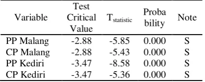
This test was conducted by using the Augmented Dickey Fuller (ADF) supported by eviews. The data was deemed as stationary if the tstatistic was lower than the test of critical value, or, if the probability was lower than 5%. Table 1 showed the result of stationary test on the data of tomato price, in the consumer context as well as in in the producer context, in Malang and Kediri Regencies.
Table 1. The Result of Stationary Test on the Data of the Consumer Price and the Producer Price
Variable
Test Critical
Value
Tstatistic Proba
bility Note
PP Malang -2.88 -5.85 0.000 S
CP Malang -2.88 -5.43 0.000 S
PP Kediri -3.47 -8.58 0.000 S
CP Kediri -3.47 -5.36 0.000 S
Specification:
The rate of error tolerance () 5% S = Stationary or significance PP = Producer price (Producer Price) CP = Consumer price (Consumer Price)
Holistically, the data regarding producer and consumer prices, in Malang and in Kediri as well, were of stationary based on the standardized level.
The Result of Heteroscedasticity Test
After the data had been already stationary, it was of urgency to examine if the data of tomato price happened to experience having heterocedasticity so that the level of volatility could be determined. The data was considered inconstantly variant (experiencing heteroscedasticity) if the obs.*R-squared was less than F-statistic. The result of examining the occurrence of heterocedasticity could be identified in the following table:
Table 2. The Result of Heteroscedasticity Test
Variable Obs.*R-squared
F-statistic Description(s) PP Malang 8.79 9,19 Not Heteroscedastic CP Malang 30.15 36,90 Not Heteroscedastic PP Kediri 18.88 21,21 Not Heteroscedastic CP Kediri 25.64 30,28 Not Heteroscedastic Specification :
PP = Producer Price CP = Consumer Price
After proving that the data of the tomato price in Malang and Kediri Regencies did not have any heteroscedasticity in 2001-2013, the next procedure was analyzing the price volatility.
The Result of Price Volatility Analysis
The rate of volatility on the tomato commodity reflected how much the level of risk the prospective economists will face is. The information related to the volatility could be employed by the economists, to be specific those who produce, consume, and sell the tomatoes as well as the government as the regulator who is to take an action.The instability of the volatility on the tomato price in the context of producers and consumers explicated that the shock that occurred was of complexity.
the context of consumers and producers throughout Malang and Kediri Regencies.
Table 3. Tomatoes’ Price Volatility in Malang and Kediri Regencies during 2001-2013
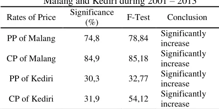
After recognizing the annual volatility, the next procedure was to measure the volatility increase for being compared to the F-Test rate so that how the volatility on the tomato price in the context of consumers and producers happened in Malang and Kediri could be simplified. The following is the significance development of the tomato price in the context of consumers and producers in Malang and Kediri:
Table 4. The Rate of Significance of the Volatility Development of the Tomato Price in Malang and Kediri during 2001 – 2013
Rates of Price Significance
(%) F-Test Conclusion PP of Malang 74,8 78,84 Significantly
increase CP of Malang 84,9 85,18 Significantly
increase PP of Kediri 30,3 32,77 Significantly
increase CP of Kediri 31,9 54,12 Significantly
increase consumers in both the regencies increased significantly. This was because the volatility increase was positive and got closer to the F-test level of the consumers. In terms of volatility, based on the context of producer or consumer, Kediri was higher than Malang.
This was due to the fact that Malang is one of the biggest tomato suppliers in East Java. As the consequence, the obtainability of the tomatoes in Malang was higher than in Kediri. The unstable obtainability (stock) of the tomatoes was reckonedas the main issue causing the continual increase of the volatility in Kediri.
The Result of Price Transmission Analysis The occurrence of the high price fluctuation is allowed to provide the sellers with chances for price manipulation so that the social welfare of the farmers go worse. For that reason, it is of importance to analyze the price transmission to identify the price increase within the context of consumers that would be projected to the producers. The method employed for analysis on the price transmission was simple regression analysis, OLS (Ordinary Least Square). This was due to the fact that the data of price variable, in general, had been of stationary in the standardized level as that of having no heteroscedasticity. In allude to the result of regression test on the price variable in the context of producers and consumers in Malang Regency, the following is the result (Table 5).
Based on Table 5, it had been identified that the coefficient of each independent variable was positive. This inferred that the independent variables affected the dependent variables. In Malang, if there was a price change in the consumer price constituting 1 rupiah, the price change in the producer price would be 0.69 rupiah. That was what would happen in the producer price
consumer price in Malang for about 1 rupiah, the consumer price in Kediri would change as well for about 0.534 rupiah.
Table 5. The Result of the Price Transmission Analysis on Tomato Price in Malang and Kediri Regencies during 2001 - 2013
Variables Established
Therefore, it could be summarized that H0 was rejected and H1 was accepted. Consequently, in Malang as that of in Kediri, there was the price transmission going from the consumer price of tomato to the producer price, and vice versa, there would be also the price transmission departing from the producer price of tomato to the consumer one.
The Result of Spillover Volatility Analysis The spillover volatility analysis was used to identify the obtainability of the volatility to be transmitted. The method used for it was GARCH method (Generalized Autoregressive Conditional Heteroscedasticity) in which it could be said as spillover volatility if the coefficient of the independent variable is positive. The variable used within the spillover measurement was the volatility
variable that had been acquired from historical volatility.
Before conducting the spillover test, the volatility variable was examined based on the aspect of stationary by means of ADF method of which heteroscedasticity was examined by using White Test. The implementation of GARCH method was by means of the program software, eviews. The GARCH method was used if the variable of the volatility was of heteroscedasticity.
After stationary and heteroscedasticity tests, it could be identified that all the volatility variables were of stationary in the first difference and of heteroscedasticity, the test of spillover volatility was executed by means of GARCH.
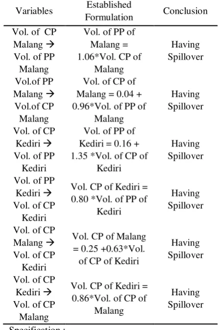
Table 6. The Result of the Spillover Volatility Analysis on Tomato Price in Malang and Kediri Regencies during 2001 - 2013
Variables Established
Vol. PP of Malang = Volatility of Producer Price in Malang
Vol. CP of Malang = Volatility of Consumer Price in Malang
Vol. PP of Kediri = Volatility of Producer Price in Kediri
Based on Table 6, it had been inspected that the coefficient of each independent variable was positive. This implicated that there was some effects of the independent variables on the dependent ones. In Malang, it showed that if there was a volatility alteration for about 1% in the consumer price, the volatility of producer price would be about 1.06%. In addition, if the volatility in the producer price increased 1%, the volatility in the consumer price would be also increased 0.96%.
Meanwhile, in Kediri, it revealed that the volatility change constituted 1% in the consumer price, the volatility change in the producer price would be 1.35%. In addition, if the volatility increased 1% for the producer price, the volatility in the consumer price would go to 0.80%. Meanwhile, in the context of consumer price of tomato between Malang and Kediri, it showed that if the volatility change constituted 1% for the consumer price in Kediri, there would be another volatility change signifying 0.63% in the consumer price of Malang. Additionally, if the volatility increased 1% in the consumer price in Malang, there would be another volatility increase for about 0.86% in the consumer price in Kediri.
Therefore, the conclusion was that H0 was rejected while H1 was accepted. As the consequently, there was a spillover in the consumer price of tomato to the producer one, and vice versa
– the spillover happened from the produce price of tomato to the consumer one.
In both the regencies, Malang and Kediri, the price change in the context of producer that had been transmitted to the context of consumer contributed much more than the price change that had been already transmitted from the consumer to the producer. Counter-productively, the volatility that was transmitted from the consumer to the producer contributed more than the volatility that was transmitted from the producer to the consumer. This implicated that the sellers held the vital role in considering the market price. The weakness of the farmers in bargaining caused the sellers tend to manipulate the price.
The active roles of the government in the stabilization of the tomato price were of urgency – one of which was by means of price transparency. This was expected that this be able to help the farmers in determining the selling price since, through the price transparency, the sellers were not be able to manipulate the price any longer.
CONCLUSION
The volatility of the tomato price in the context of consumer and producer in Malang during 2001 – 2013 increased significantly. This was based on the volatility measurement that revealed the positive alteration in terms of producer price volatility, constituting 74.8% and of which rate approached the f-test, 78.84. Meanwhile, in the context of consumer, the development rate showed the positivity, signifying 84.9% and the rate advanced the f-test, constituting 85.18. On the other hands, the volatility on the consumer and producer prices of tomato in Kediri during Kediri 2001 – 2013 went up significantly. This was referred to the volatility that exhibited the positive development on the producer price volatility, signifying 30.3% of which rate loomed the f-test score, 32.77. Meanwhile, in the consumer context, the development rate showed positivity, 31.9%, of which f-test rate constituted 54.12.
The price transmission happened on the tomato price in the context of consumer and also the producer, both in Malang and Kediri. In addition, there was also the price transmission from the tomato price in the context of producer to the context of consumer in both the regencies, Malang and Kediri. This was represented by the result of regression test in which each the coefficients showed the positive results.
The spillover volatility happened in tomato price in Malang as that of in Kediri, in the context of producer and consumer. It was proved by the coefficient of GARCH that was positive. This implicated that the volatility of the price in each price rate was transmitted.
The price transmission did much happen in tomato markets, operating in Malang as well as in Kediri. This was due to the regression coefficient that was positive. In addition, the spillover occurred in Malang and Kediri markets. This was proved by the GARCH coefficient that was positive as well.
REFERENCES
Anindita, R. and Baladina, N. (2016). Pemasaran Produk Pertanian (Marketing of Farming Products). Andi Offset. Yogyakarta
Gilbert, C. L. and C. W. Morgan. (2011). Methods to Analyze Agricultural Commodity Price Volatility. Springer
Analyze Price Volatility. Spring Science and Business Media, LLC. Europe.
Buguk, C., D Hudson., T. Hanson. (2003). Price Volatility Spillover in Agricultural Markets: An Examination of U.S. Catfish Markets. Journal of Agricultural and Resource Economics 28(1): 86-99. Gaziosmanpasa University. Turkey