The Simulation Study to Test the Performance of Quantile
Regression Method With Heteroscedastic Error Variance
Ferra Yanuar1*, Laila Hasnah2, Dodi Devianto3
1,2,3Jurusan Matematika FMIPA Universitas Andalas Kampus Limau Manis 25163 Padang
* Corresponding Author. E-mail: [email protected]
ABSTRACT
Least square estimator has many limitations. This estimator will not be a Best Linear Unbiased Estimator (BLUE) in the condition of the variance error term have heteroscedasticity problem. Quantile regression is a robust approach in situations where the limitation addressed above present for least square estimator. The purpose of this study is to describe the performance of quantile regression method in modeling a data set which contain the heteroscedasticity problem. To achieve the goal, a data set is generated and statistical framework quantile method then applied to the data. The consistency of the proposed model is then checked by doing a simulation study. This study proves that the quantile regression method is able to produce acceptable parameter model since the proposed models have large Pseudo R2 and small mean square error (MSE) for all parameter estimated. It could be conclude here that quantile regression method is an unbiased estimator method and able to result acceptable model althought in the present of heteroscedasticity problem of variance error.
Keywords: Heteroscedasticity, quantile regression, simulation study, Pseudo R2, mean square error (MSE).
INTRODUCTION
In modeling the relationship between covariates and responses, it need estimator method to estimate the parameter model. To estimate the value of parameters, it usually use the Ordinary Least Squares (OLS). The principle of this method is to minimize the sum of the squares of the error. This OLS is applied if all model assumptions are met (independent observations, linearity of conditional means, normality of response variable and homogeneity of error variance). In all model assumptions are met, the estimator method is called as BLUE (Best Linear Unbiased Estimator). However, if one or more of the assumptions are not met, the results could be misleading [1].
In regression, an error is how far a point deviates from the regression line. Ideally, our data should be homoscedastic (i.e. the variance of the errors should be constant). In many real world applications, this situation rarely happens. Most data is heteroscedastic by nature. Due to these limitatios, an alternative approach to classical linear regression is in demand. Quantile regression is a robust approach in situations where the limitations addressed above [2] present for ordinary least square estimator.
regression in his theory is able to overcome the violation of normality assumptions, heteroscedasticity, multicollinearity problems and so on. This method uses the parameter estimation approach by separating or dividing the data into quantities, by assuming the conditional quantization function on a distribution of data and minimizing the absolute asymmetry of unsymmetric weighted error and presupposes a conditional quantile function on a distribution of data [5].
In this paper, we adopt the quantile regression approach to modeling groups of data with non homogeneity of error variance. Section 2 of the paper, describes the theoretical framework of quantile regression and its indicators to determine the goodness of fit of the proposed model. In section 3, we illustrate the implementation of quantile regression through a simulated case-study. We choose two covariates in our model hypothesis.as the predictors to the response variable. We end with a short discussion in Section 4.
FUNDAMENTAL THEORIES AND RELATED WORKS
In stricly linear models, a simple approach to estimating the conditional quantiles is suggested in Koenker and Basset [2]. Based on the classical regression model, we have:
𝑦𝑖 = 𝒙𝒊′𝜷 + 𝜀𝑖, 𝑖 = 1,2, … , 𝑛 (1)
The prediction based on the median, that is, by minimizing the absolute number of errors can be written using following equation :
𝑚𝑖𝑛 ∑𝑛𝑖=1|𝑦𝑖− 𝑦̂|𝑖 2 (3) Furthermore, the linear equations for -th quantil can be written as follows : 𝑦𝑖 = 𝒙𝒊′𝜷𝝉+ 𝜀𝑖, 𝑖 = 1,2, . . , 𝑛 (4)
Noted that 𝑦̂ = 𝒙𝑖 𝒊′𝜷𝝉, the parameter estimate for th quantile is to minimize the absolute
value of the error by weighting τ for the positive and weighted error (1- τ) for the negative error [4]. The 𝜏th (0 < 𝜏 < 1) quantile of 𝜀𝑖 is the value, 𝑄𝜏, for which 𝑃 (𝜀𝑖 < 𝑄𝑌(𝜏)) = 𝜏. The 𝜏th Equivalently, we may rewrite (5) as :
𝑚𝑖𝑛𝛽𝜖ℛ{∑𝑖=1𝑛 𝜏|𝑦𝑖− 𝒙𝒊′𝜷𝝉| + ∑ (1 − 𝜏)|𝑦𝑛𝑖=1 𝑖− 𝒙𝒊′𝜷𝝉|} (7)
The meaning which can be added to explain the equation (7), namely that all observations greater than the quantile value, multiplied by the weighting τ and the observations whose value is less than the quantile multiplied by 1 − 𝜏.
2.2 Goodness of Fit using Pseudo R2
The indicator of the goodness of fit for the model can be predicted with Pseudo R2 as defined below [2]:
Pseudo 𝑅𝜏2= 1 −𝑅𝐴𝑊𝑆𝜏
𝑇𝐴𝑆𝑊𝜏 (9)
where :
𝑅𝐴𝑊𝑆𝜏 = ∑ 𝜏|𝑦𝑖− 𝛽̂0(𝜏) − 𝛽̂1(𝜏)𝒙𝒊− ⋯ − 𝛽̂𝑛(𝜏)𝒙𝒊| 𝑦𝑖≥𝛽̂0(𝜏)+𝛽̂1(𝜏)𝒙𝒊+⋯+𝛽̂𝑛(𝜏)𝒙
+ ∑𝑦𝑖<𝛽̂0(𝜏)+𝛽̂1(𝜏)𝒙𝒊+⋯+𝛽̂𝑛(𝜏)𝒙(1 − 𝜏)|𝑦𝑖− 𝛽̂0(𝜏) − 𝛽̂1(𝜏)𝒙𝒊 − 𝛽̂𝑛(𝜏)𝒙𝒊|
(10) and
𝑇𝐴𝑆𝑊𝜏= ∑𝑦𝑖≥𝜏𝜏|𝑦𝑖− 𝜏̂| +∑𝑦𝑖<𝜏(1 − 𝜏)|𝑦𝑖− 𝜏̂| (11)
The value of 𝑅𝐴𝑊𝑆𝜏 (Residual Absolute Sum of Weighted) is always less than the value of 𝑇𝐴𝑆𝑊𝜏 (Total Absolute Sum of Weighted) so that the Pseudo 𝑅𝜏2 will be in the range 0 to 1. The closer the Pseudo R2 value to one the model will be better. However, the virtues of Pseudo R2 can not be used to test the overall goodness of fit for the model, it can only be used to test the merits of the selected quantile [1,2].
2.3 Mean Square Error (MSE)
The parameter estimate obtained is said to be good if it has a small bias and small variance. Therefore, to see the goodness of estimating the parameters based on the bias and variance values simultaneously, represented in the value of Mean Square Error (MSE) [8, 9, 10], formulated as follows :
𝑀𝑆𝐸(𝛽̂𝑗(𝜏𝑞)) = 𝑉𝑎𝑟 ((𝛽̂𝑗(𝜏𝑞)) + 𝐵𝑖𝑎𝑠 (𝛽̂𝑗(𝜏𝑞))2 (12) where :
𝑀𝑆𝐸(𝛽̂𝑗(𝜏𝑞)) : value of MSE for 𝑗 = 1,2, … 𝑝 𝜏𝑞 = 𝑞𝑢𝑎𝑛𝑡𝑖𝑙 𝑞 = 1,2, … , 𝑘 𝑉𝑎𝑟 ((𝛽̂𝑗(𝜏𝑞)) : variance for selected quantile
𝑉𝑎𝑟 ((𝛽̂𝑗(𝜏𝑞)) =𝑛 ∑ (𝛽̂𝑗(𝜏𝑞))
2 𝑛
𝑖=1 −(∑𝑛𝑖=1(𝛽̂𝑗(𝜏𝑞)))2
𝑛(𝑛−1)
𝐵𝑖𝑎𝑠 (𝛽̂𝑗(𝜏𝑞)) : the value of bias for selected quantile is obtained from the mean of the difference of the expected value and the estimated value, or :
𝐵𝑖𝑎𝑠 (𝛽̂𝑗(𝜏𝑞)) =𝑛1∑𝑛𝑖=1((𝛽̂𝑗(𝜏𝑞)) −(𝛽𝑗(𝜏𝑞))
RESULT AND DISCUSSION
We describe our approach to quantile regression by conducting the simulation study. In this research, we design two covariates each measuring 100 samples. The response variable, 𝑦𝑖 is generated from the model :
𝑦𝑖 = 𝛽0+ 𝛽1𝑥𝑖1+ 𝛽2𝑥𝑖2+ 𝜀𝑖, 𝑖 = 1, … ,100 (13)
where covariate 𝑥𝑖1 is generated from a standard normal distribution and 𝑥𝑖2 is generated from exponential with one degrees of freedom. The parameter 𝛽0, 𝛽1 and 𝛽2 are set to 1.2, 1, and 1.7 respectively. The data for error is also generated by taking the mean at zero and its variances have heteroscedasticity problems. We consider the heteroscedastic normal, 𝑁(0, √0.01 x (𝑿𝜷)2) for distribution of error term.
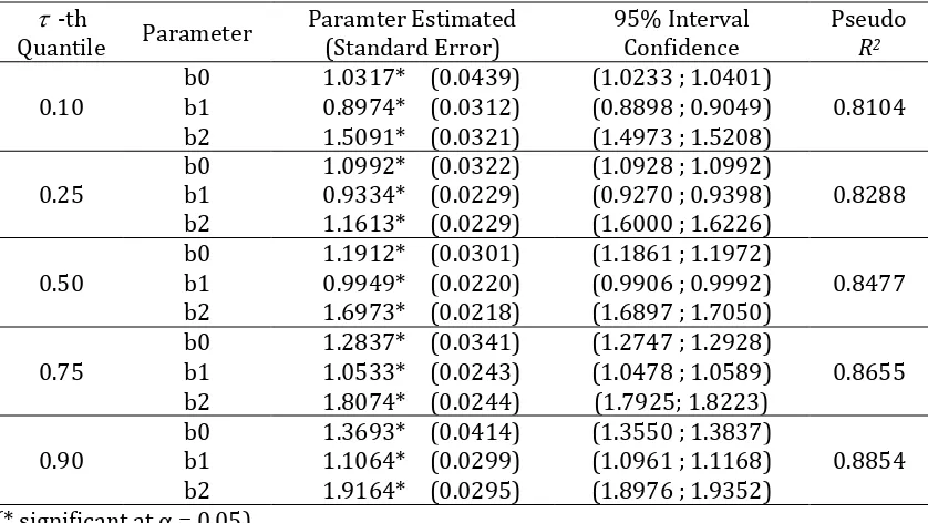
Table 1. Quantile Regression Estimates
𝜏th Quantile Parameter Estimates Standard error
0.10
The next analysis in the quantile regression is a consistency test of the proposed model to reveal the performance of the quantile approach and its associated algorithm in recovering the true parameters of the quantile regression analysis. Consistency test is done by doing simulation study. Simulation study does so by generating a set of new data set by sampling with replacement
from the original data set, and fitting the model to each new data set [11, 12]. To compute standard
errors for calculating the 95% confidence interval of all parameters in this study, roughly 25
model fits are determined. The goodness of fit of each model are also calculated. Table 2 presents the result taken from the simulation study.
Table 2. Simulation Results of 25 Data Sets Using Quantile Regression Approach
consider the 50th quantile, the estimated value for 𝛽̂0, 𝛽̂1 and 𝛽̂2 are 1.1916, 0.9949, and 1.6973 respectively. Based on Table 2, we also know that all parameter estimated values fall within 95% confidence intervals obtained from the simulation study. It means quantile 95% confidence interval seem to work well here and parameter estimated are acceptable.
The goodness of fit for the each quantile regression model is presented by the value of Pseudo R2, shown in the last column in Table 2. All Pseudo R2 values obtained here are more than 80%, indicating that all proposed model are adequate and could be accepted.
In this study we also determine the value of of MSE (Mean Square Error) to ensure that parameter estimated have small bias and small variance. Table 3 below presents the MSE value of the quantile regression method for all three parameter estimated at corresponding quantile points. results indicate that quantile regression method is able to produce unbiased parameter model since it has small bias and small variance.
Based on any results here, we could believe that the power of our quantile regression method result the best fit for the model althought in the existence of heteroscedastic error variance.
CONCLUSIONS
This present study purposes to describe the performace of quantile regression method in modeling the data containing non-uniform variance problem (heteroscedasticity). A data set with two covariates is generated, each measuring 100 samples. The distribution for error term is heteroscedastic normal, 𝑁(0, √0.01 x (𝑿𝜷)2) is designed to generate a response variable. Each parameter model are also set as initial values. A simulation study is done to check the power of quantile regression algorithm.
This study resulted that all parameter estimated are close to the initial values. The value of Pseudo R2 for all proposed model at any selected quantile points are quite large, more than 80%. Based on simulation study, the value of parameter estimated are within 95% confidence intervals indicating that parameter estimated could be accepted. This study also result that quantile regression method is able to produce small value of MSE. Therefore, it could be concluded here that quantile regression methods is unbiased estimator method and could result the acceptable model although in the due of heteroscedasticity problem of error variance.
REFERENCES
[1] Ferra Y, Hazmira Y and Izzati R. 2016. Penerapan Metode Regresi Kuantil pada Kasus Pelanggaran Asumsi Kenormalan Sisaan. Eksakta, 1 (XVII) : 33 – 37.
[2] Davino C, Furno M, and Vistocco D. 2014. Quantile Regression: Theory and Applications. John Wiley & Sons, Ltd.
[3] Arbia, G. 2006. Spatial Econometrics: Statistical Foundation Application to Regional Convergence. Springer, Berlin
[4] Koenkar.R. and Basset,G.Jr.1978. Quantiles Regression. Econometrica. 46. 33-50
[5] Kozumi H and Kobayashi G. 2011. Gibbs sampling methods for Bayesian quantile regression. Journal of Statistical Computation and Simulation, 81 (11) : 1565 – 1578. [6] Feng X and Zhu L. 2016. Estimation and Testing of Varying Coefficients in Quantile
[7] Yanuar F. 2013. Quantile Regression Approach to Determine the Indicator of Health Status. Scientific Research Journal , I (IV): 17 – 23.
[8] Yang Y, Wang HJ and He X. 2015. Posterior inference in Bayesian quantile regression with asymmetric Laplace likelihood. International Statistical Review, 0 0, 1-18 doi: 10.1111.insr.12114
[9] He X. and Zhu LX. 2011. A lack of fit test for quantile regression. Journal of the American Statistical Association, 98 (464) : 1013 - 1022
[10] Feng, X., He, X., and Hu, J. 2011. Wild Boostrap for Quantile Regression. Biometrica, 98, 995–999.
[11] Yanuar F, Ibrahim K and Jemain AA. 2013. Bayesian structural equation modeling index in the health model. Journal of Applied Statistics, 40 (6) : 1254–1269.