Deep Neural
Networks in Machine
Translation: An
Overview
Jiajun Zhang and Chengqing Zong, Institute of Automation, Chinese Academy of Sciences
Deep neural
networks (DNNs)
are increasingly
popular in machine
translation.
symbol variable processing, such as natural language processing (NLP). As one of the more challenging NLP tasks, machine trans-lation (MT) has become a testing ground for researchers who want to evaluate various kinds of DNNs.
MT aims to find for the source language tence the most probable target language sen-tence that shares the most similar meaning. Essentially, MT is a sequence-to-sequence pre-diction task. This article gives a comprehen-sive overview of applications of DNNs in MT from two views: indirect application, which at-tempts to improve standard MT systems, and direct application, which adopts DNNs to de-sign a purely neural MT model. We can elabo-rate further:
• Indirect application designs new features with DNNs in the framework of standard MT systems, which consist of multiple sub-models (such as translation selection and lan-guage models). For example, DNNs can be leveraged to represent the source language
context’s semantics and better predict trans-lation candidates.
• Direct application regards MT as a se-quence-to-sequence prediction task and, without using any information from stan-dard MT systems, designs two deep neural networks—an encoder, which learns con-tinuous representations of source language sentences, and a decoder, which generates the target language sentence with source sentence representation.
Let’s start by examining DNNs themselves.
Deep Neural Networks
Researchers have designed many kinds of DNNs, including deep belief networks (DBNs), deep stack networks (DSNs), con-volutional neural networks (CNNs), and recurrent neural networks (RNNs). In NLP, all these DNNs aim to learn the syntactic and semantic representations for the dis-crete words, phrases, structures, and sen-tences in the real-valued continuous space so
D
ue to the powerful capacity of feature learning and representation, deep
neural networks (DNNs) have made big breakthroughs in speech
recog-nition and image processing. Following recent success in signal variable
that similar words (phrases or struc-tures) are near each other. We briefly introduce five popular neural networks after giving some notations—namely, we use wi to denote the ith word of a T-word sentence, and xi as the cor-responding distributed real-valued vector. Vectors of all the words in the vocabulary form the embedding matrix L ∈ Rk×|V|, where k is the
embedding dimension and |V| is the vocabulary size. Additionally, U and W are parameter matrices of a neural network, and b is the bias; f and e in-dicate the source and target sentence, respectively.
Feed-Forward Neural Network
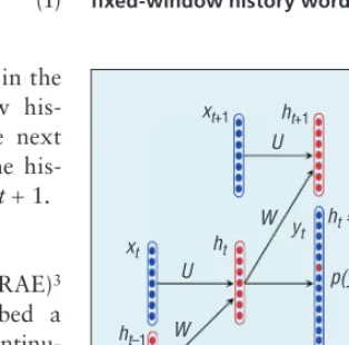
The feed-forward neural network (FNN) is one of the simplest multilayer net-works.1 Figure 1 shows an FNN
ar-chitecture with hidden layers as well as input and output layers. Taking the language model as an example, the FNN attempts to predict the conditional probability of the next word given the fixed-window history words. Suppose we have a T-word sentence, w1, w2, ..., wt, ..., wT; our task is to estimate the four-gram conditional probability of wt given the trigram history wt−3, history. The hidden layers are followed
to extract the abstract representation of the history words through a linear transformation W × xt_history and a
non-linear projection f(W × xt_history + b),
such as f=tanh (x)). The softmax layer is usually adopted in the output to predict each word’s probability in the vocabulary.
Recurrent Neural Network
The recurrent neural network (Recur-rentNN)2 is theoretically more
power-ful than FNN in language modeling due
to its capability of representing all the history words rather than a fixed-length context as in FNN. Figure 2 depicts the RecurrentNN architecture. Given the history representation ht−1 encoding all
the preceding words, we can obtain the new history representation ht with the formula ht=Uxt +Wht−1. With ht, we can calculate the probability of next word using the softmax function:
p y e vocabulary. Similarly, the new his-tory representation ht and the next word will be utilized to get the his-tory representation ht+1 at time t+ 1.
Recursive Auto-encoder
The recursive auto-encoder (RAE)3
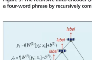
provides a good way to embed a phrase or a sentence in continu-ous space with an unsupervised or semisupervised method. Figure 3 shows an RAE architecture that learns a vector representation of a four-word phrase by recursively combining two children vectors in a bottom-up man-ner. By convention, the four words w1, w2, w3, and w4 are first projected into
real-valued vectors x1, x2, x3, and x4.
In RAE, a standard auto-encoder (in box) is reused at each node. For two children c1=x1 and c2=x2, the
auto-encoder computes the parent vector y1
as follows:
y1=f(W(1) [c1; c2] +b(1)). (2)
To assess how well the parent’s vec-tor represents its children, the standard auto-encoder reconstructs the children in a reconstruction layer:
[c′1; c′2] =f′(W(2)y1+b(2)). (3)
The standard auto-encoder tries to minimize the reconstruction errors
between the inputs and the recon-structions during training:
Erec([c1; c2]) = ½ ||[c1; c2] - [c′1; c′2]||2.
(4)
The same auto-encoder is reused until the whole phrase’s vector is gen-erated. For unsupervised learning, the objective is to minimize the sum of reconstruction errors at each node in the optimal binary tree:
RAE x E c c
Figure 1. The feed-forward neural network (FNN) architecture. Taking the language model as an example, the FNN attempts to predict the conditional probability of the next word given the fixed-window history words.
Hidden layers
Input W 2
W 1
Figure 2. The recurrent neural network (RecurrentNN) architecture. Theoretically, it’s more powerful than FNN in language modeling due to its capability of representing all the history words rather than a fixed-length context.
N A T U R A L L A N G U A G E P R O C E S S I N G
A(x) denotes all the possible binary trees that can be built from input x.
Recursive Neural Network
The recursive neural network (Recur-siveNN)4 performs structure prediction
and representation learning using a bot-tom-up fashion similar to that of RAE. However, RecursiveNN differs from RAE in four points: RecursiveNN is op-timized with supervised learning; the tree structure is usually fixed before train-ing; RecursiveNN doesn’t have to recon-struct the inputs; and different matrices
can be used at different nodes. Figure 4 illustrates an example that applies three different matrices. The structure, repre-sentation, and parameter matrices W(1), W(2), and W(3) have been learned to
op-timize the label-related supervised objec-tive function.
Convolutional Neural Network
The convolutional neural network (CNN)5consists of the convolution and
pooling layers and provides a standard architecture that maps variable-length sentences into fixed-size distributed vec-tors. Figure 5 shows the architecture. The CNN model takes as input the sequence of word embeddings, sum-marizes the sentence meaning by con-volving the sliding window and pooling the saliency through the sentence, and yields the fixed-length distributed vector with other layers, such as drop-out and fully connected layers.
Given a sentence w1, w2, ..., wt, ..., wT, each word wt is first projected into a vector xt. Then, we concate-nate all the vectors to form the input X= [x1, x2, ..., xt, ..., xT].
The convolution layer involves sev-eral filters W ∈ Rh×k that summarize the
information of an h-word window and produce a new feature. For the window of h words Xt:t+h−1, a filter Fl (1 ≤l ≤ L) generates the feature ytl as follows:
ytl =f WX
(
t t h:+ −1+b)
. (6)When a filter traverses each window from X1:h−1 to XT−h+1:T, we get the
fea-ture map’s output: y y1l, 2l,…,yT tl− +1
(yl ∈ RT−h+1). Note that the sentences
differ from each other in length T, and yl has different dimensions for different sentences. A key question becomes how do we transform the variable-length vector yl into a fixed-size vector?
The pooling layer is designed to perform this task. In most cases, we apply a standard max-over-time pool-ing operation over yl and choose the
maximum value yˆl=max y
{ }
l . WithL filters, the dimension of the pooling layer output will be L. Using other ers, such as fully connected linear lay-ers, we can finally obtain a fixed-length output representation.
Machine Translation
Statistical models dominate the MT community today. Given a source lan-guage sentence f, statistical machine translation (SMT) searches through all the target language sentences e and finds the one with the highest probability:
′=
e p e f
e
arg max ( | ). (7)
Usually, p(e|f) is decomposed using the log-linear model6:
′=
=
(
∑
(
)
)
∑
′e p e f
exp h f e
e
e
i i i
e arg max ( | )
arg max
,
λ
eexp h f e i i i
∑
(
′)
(
λ ,)
, (8) y3 =f(W(1)[y
2; x4]+b)
y2 =f(W(1)[y 1; x3]+b)
y1 =f(W(1)[x 1; x2]+b)
x1 x2 x3 x4
Figure 3. The recursive auto-encoder (RAE) architecture. It learns a vector representation of a four-word phrase by recursively combining two children vectors in a bottom-up manner.
Figure 4. Recursive neural network (RecursiveNN) architecture. The structure, representation, and parameter matrices W(1), W(2), and W(3)
have been learned to optimize the label-related supervised objective function.
y3 =f(W (3)[y2; x4]+b(3))
label
label
label
y2 =f(W (2)[y1; x3]+b(2))
x2
x1 x3 x4
where hi(f, e) can be any translation fea-ture and λi is the corresponding weight. The translation process can be di-vided into three steps: partition the source sentence (or syntactic tree) into a sequence of words or phrases (or set of subtrees), perform word/phrase or subtree translation; and compos-ite the fragment translations to obtain the final target sentence. If the transla-tion unit is word, it’s the word-based model. If phrase is the basic transla-tion unit, it’s the popular phrase-based model. In this article, we mainly take the phrase-based SMT7 as an example.
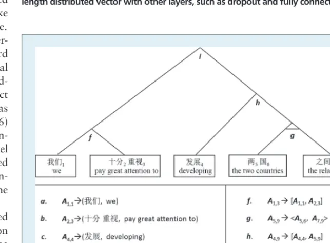
In the training stage, we first per-form word alignment to find word correspondence between the bilingual sentences. Then, based on the word-aligned bilingual sentences, we extract phrase-based translation rules (such as the a–e translation rules in Figure 6) and learn their probabilities. Mean-while, the phrase reordering model can be trained from the word-aligned bilingual text. In addition, the lan-guage model can be trained with the large-scale target monolingual data.
During decoding, the phrase-based model finds the best phrase partition of the source sentence, searches for the best phrase translations, and figures out the best composition of the target phrases. Figure 6 shows an example for a Chinese-to-English translation. Phrasal rules (a–e) are first utilized to get the partial translations, and then reordering rules (f–i) are employed to arrange the translation positions. Rule g denotes that “the two countries” and “the relations between” should be swapped. Rules f, g, and i just compos-ite the target phrases monotonously. Finally, the language model measures which translation is more accurate.
Obviously, from training and decod-ing, we can see the difficulties in SMT:
• It’s difficult to obtain accurate word alignment because we have
no knowledge besides the parallel data.
• It’s difficult to determine which tar-get phrase is the best candidate for a source phrase because a source phrase can have many translations, and different contexts lead to differ-ent translations.
• It’s tough work to predict the trans-lation derivation structure because phrase partition and phrase reor-dering for a source sentence can be arbitrary.
• It’s difficult to learn a good language model due to the data sparseness problem.
V
ariable-length sentence
e
L
L
Figure 5. The convolutional neural network (CNN) architecture. The CNN model takes as input the sequence of word embeddings, summarizes the sentence meaning by convolving the sliding window and pooling the saliency through the sentence, and yields the fixed-length distributed vector with other layers, such as dropout and fully connected layers.
N A T U R A L L A N G U A G E P R O C E S S I N G
The core issues lie in two areas: data sparseness (when considering addi-tional contexts) and the lack of se-mantic modeling of words (phrases and sentences). Fortunately, DNNs are good at learning semantic representa-tions and modeling wide context with-out severe data sparseness.
DNNs in Standard SMT Frameworks
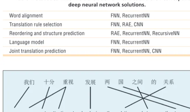
The indirect application of DNNs in SMT aims to solve one difficult prob-lem in an SMT system with more accurate context modeling and syn-tactic/semantic representation. Table 1 gives an overview of SMT problems and their various DNN solutions.
DNNs for Word Alignment
Word alignment attempts to identify the word correspondence between parallel sentence pairs. Given a source sentence f=f1, f2, ..., ft, ..., fT and its target translation e =e1, e2, ..., et, ..., eT′, the word alignment is to find the set A = {(i, j), 1 ≤ i ≤ T, 1 ≤ j ≤ T′}, in which (i, j) denotes that fi and ej are translations of each other. Figure 7 shows an example.
In SMT, the generative model is a popular solution for word alignment. Generative approaches use the statistics
of word occurrences and learn their pa-rameters to maximize the likelihood of the bilingual training data. They have two disadvantages: discrete symbol representation can’t capture the simi-larity between words, and contextual information surrounding the word isn’t fully explored.
Nan Yang and colleagues8 extended
the HMM word alignment model and adapted each subcomponent with an FNN. The HMM word alignment takes the following form:
p a e f plexej f p aa d j a j
T
j j
( , | )= ( | ) ( − )
−
= ′
∏
11
,
(9)
where plex is the lexical translation
probability and pd is the distor-tion probability. Both components are modeled with an FNN. For the lexical translation score, the authors employed the following formula:
slex(ej|fi, e, f) = f3° f2° f1° L
(window(ej), window (fi)). (10)
The FNN-based approach considers the bilingual contexts (window(ej) and window (fi)). All the source and target words in the window are mapped into vectors using L∈ Rk×|V| and concatenated
to feed to hidden layers f1 and f2.
Finally, the output layer f3 generates
a translation score. A similar FNN is applied to model the distortion score sd(aj- aj−1). This DNN-based method
not only can learn the bilingual word embedding that captures the similarity between words, but can also make use of wide contextual information.
Akihiro Tamura and colleagues9
adopted RecurrentNN to extend the based model. Because the FNN-based approach can only explore the context in a window, the Recur-rentNN predicts the jth alignment aj by conditioning on all the preceding alignments a1j−1.
The reported experimental results indicate that RecurrentNN outper-forms FNN in word alignment qual-ity on the same test set. It also implies that RecurrentNN can capture long dependency by trying to memorize all the history.
DNNs for Translation Rule Selection
With word-aligned bilingual text, we can extract a huge number of transla-tion rules. In phrase-based SMT, we can extract many phrase translation rules for a given source phrase. It becomes a key issue to choose the most appropri-ate translation rules during decoding. Traditionally, translation rule selection is usually performed according to co-occurrence statistics in the bilingual training data rather than by exploring the large context and its semantics.
Will Zou and colleagues10 used two
FNNs (one for source language and the other for target language) to learn bilingual word embeddings so as to make sure that a source word is close to its correct translation in the joint embedding space. The FNN used for source or target language takes as in-put the concatenation of the context words, applies one hidden layer, and finally generates a score in the output
Table 1. Statistical machine translation difficulties and their corresponding deep neural network solutions.
Word alignment FNN, RecurrentNN
Translation rule selection FNN, RAE, CNN
Reordering and structure prediction RAE, RecurrentNN, RecursiveNN
Language model FNN, RecurrentNN
Joint translation prediction FNN, RecurrentNN, CNN
we pay great attention to developing the relations between the two countries
Jsrc+lJtgt→src, (11)
where Jsrc is the contrastive objective
function with monolingual data, and Jtgt→src is a bilingual constraint:
Jtgt→src=|| Lsrc - Atgt→srcLtgt||2. (12)
Equation 12 says that after word alignment projection Atgt→src, the
tar-get word embeddings Ltgt should be
close to the source embeddings Lsrc.
This method has shown that it can cluster bilingual words with similar meanings. The bilingual word embed-dings are adopted to calculate the se-mantic similarity between the source and target phrases in a phrasal rule, effectively improving the performance of translation rule selection.
Jianfeng Gao and colleagues11
at-tempted to predict the similarity be-tween a source and a target phrase using two FNNs with the objective of maximizing translation quality on a validation set. For a phrasal rule (f1,…,i, e1,…,j), the FNN (for source or target language) is employed first to abstract the vector representa-tion for f1,…,i and e1,…,j, respectively. The similarity score will be score
f1, ,…i,e1, ,…j yf1, ,iTye1, ,j
… …
(
)
= . The FNNparameters are trained to optimize the score of the phrase pairs that can lead to better translation quality in the valida tion set.
Because word order isn’t considered in the above approach, Jianjun Zhang and colleagues12 proposed a bilingually
constrained RAE (BRAE) to learn se-mantic phrase embeddings. As shown in Figure 3, unsupervised RAE can get the vector representation for each phrase. In contrast, the BRAE model not only tries to minimize the reconstruction error but also attempts to minimize the semantic distance between phrasal
learn the semantic vector representation for each source and target phrase. Using BRAE, each phrase translation rule can be associated with a semantic similarity. With the help of semantic similarities, translation rule selection is much more accurate.
Lei Cui and colleagues13 applied the
auto-encoder to learn the topic repre-sentation for each sentence in the par-allel training data. By associating each translation rule with topic informa-tion, topic-related rules can be selected according to the distributed similarity with the source language text.
Although these methods adopt dif-ferent DNNs, they all achieve better rule prediction by addressing differ-ent aspects such as phrase similar-ity and topic similarsimilar-ity. FNN as used in the first two approaches is simple and learns much of the semantics of words and phrases with bilingual or BLEU (Bilingual Evaluation Under-study) objectives. In contrast, RAE is capable of capturing a phrase’s word order information.
DNNs for Reordering and Structure Prediction
After translation rule selection, we can obtain the partial translation candidates for the source phrases (see the branches in Figure 6). The next task is to perform derivation structure prediction, which includes two subtasks: determining which two neighboring candidates should be composed first and deciding how to compose the two candidates. The first subtask hasn’t been explicitly modeled to date. The second subtask is usually done via the reordering model. In SMT, the phrase reordering model is formalized as a classification problem, and discrete word features are employed, although data sparse-ness is a big issue and similar phrases
Peng Li and colleagues adopted the semisupervised RAE to learn the phrase representations that are sensitive to reordering patterns. For two neigh-boring translation candidates (f1, e1)
and (f2, e2), the objective function is
E=aErec(f1, e1, f2, e2) + (1 - a) Ereorder
((f1, e1), (f2, e2)), (13)
where Erec(f1, e1, f2, e2) is the sum
of reconstruction errors, and Ereorder
((f1, e1), (f2, e2)) is the reordering loss
computed with cross-entropy error function. The semisupervised RAE shows that it can group the phrases sharing similar reordering patterns.
Feifei Zhai and colleagues16 and
Jianjun Zhang and colleagues17
explic-itly modeled the translation process of the derivation structure prediction. A type-dependent RecursiveNN17
jointly determines which two partial translation candidates should be com-posed together and how that should be done. Figure 8 shows a training exam-ple. For a parallel sentence pair (f, e), the correct derivation exactly leads to e, as Figure 8a illustrates. Meanwhile, we have other wrong derivation trees in the search space (Figure 8b gives one incor-rect derivation). Using RecursiveNN, we can get scores SRecursiveNN(cTree)
and SRecursiveNN(wTree) for the correct
and incorrect derivations. We train the model by making sure that the score of the correct derivation is better than that of incorrect one:
SRecursiveNN(cTree) ≤ SRecursiveNN(wTree)
+ D(SRecursiveNN(cTree),
SRecursiveNN(wTree)), (14)
where, D( SRecursiveNN(cTree), SRecursiveNN
(wTree)) is a structure margin.
N A T U R A L L A N G U A G E P R O C E S S I N G
combining RecursiveNN and Recur-rentNN together. This not only retains the capacity of RecursiveNN but also takes advantage of the history.
Compared to RAE, RecursiveNN ap-plies different weight matrixes according to different composition types. Other work17 has shown via experiments that
RecursiveNN can outperform RAE on the same test data.
DNNs for Language Models in SMT
During derivation prediction, any composition of two partial tions leads to a bigger partial transla-tion. The language model performs the task to measure whether the transla-tion hypothesis is fluent. In SMT, the
most popular language model is the count-based n-gram model. One big issue here is that data sparseness be-comes severe as n grows. To alleviate this problem, researchers tried to de-sign a neural network-based language model in the continuous vector space.
Yoshua Bengio and colleagues1
de-signed an FNN as Figure 1 shows to learn the n-gram model in the continu-ous space. For an n-gram e1, ..., en, each word in e1, ..., en−1 is mapped onto a
vector and concatenation of vectors feed into the input layer followed by one hidden layer and one softmax layer that outputs the probability p(en|e1, ..., en−1).
The network parameters are optimized to maximize the likelihood of the
large-scale monolingual data. Ashish Vaswani and colleagues19 employed two hidden
layers in the FNN that’s similar to Bengio’s FNN.
The n-gram model assumes that the word depends on the previous n - 1 words. RecurrentNN doesn’t use this assumption and models the probabil-ity of a sentence as follows:
p e eT p ej e ej j
T
1 1 1
1
,…, ′ | ,…, − .
= ′
(
)
=∏
(
)
(15)
All the history words are applied to predict the next word.
Tomas Mikolov20 designed the
Re-currentNN (see Figure 2). A sentence start symbol <s> is first mapped to a real-valued vector as h0 and then
em-ployed to predict the probability of e1; h0 and e1 are used to form the new
his-tory h1 to predict e2, h1 and e2
gener-ate h2, and so on. When predicting eT′, all the history e1, ..., eT′−1 can be used.
The RecurrentNN language model is employed to rescore the n-best trans-lation candidates. Michael Auli and Jianfeng Gao21 integrated the
Re-currentNN language model during the decoding stage, and further im-provements can still be obtained than just rescoring the final n-best transla-tion candidates.
DNNs for Joint Translation Prediction
The joint model predicts the target translation by using both of the source sentences’ information and the target-side history.
Yuening Hu and colleagues22 and
Youzheng Wu and colleagues23 cast the
translation process as a language model prediction over the minimum transla-tion units (smallest bilingual phrase pairs satisfying word alignments). They adopted RecurrentNN to model the process.
Michael Auli and colleagues24 adapted
the RecurrentNN language model and
Figure 8. Type-dependent RecursiveNN: (a) correct derivation vs. (b) incorrect derivation. The correct derivation is obtained by performing forced decoding on the bilingual sentence pair; the derivation structure leads directly to the correct translation. The incorrect derivation is obtained by decoding the source sentence with the trained SMT model; it results in a wrong translation.
developing the relations between the two countries
the relations between the two countries
developing the two countries
the two countries
the relations between
between the relations developing the two countries between the relations
developing the two countries
developing
M
M
(a) Correct derivation tree
(b) Wrong derivation tree M
added a vector representation for the source sentence as the input along with the target history. Jacob Devlin and col-leagues25 proposed a neural network
joint model (NNJM) that adapts FNN to take as input both the n - 1 target word history and h-window source con-text. They reported promising improve-ments over the strong baseline. Because no global information is employed in NNJM, Fandong Meng and colleagues26
and Jiajun Zhang and colleagues27
pre-sented an augmented NNJM model: CNN is designed to learn the vector representation for each source sentence; then, the sentence representation aug-ments the NNJM model’s input to pre-dict the target word generation. This approach further improves the transla-tion quality over the NNJM model.
The RecurrentNN joint model just fits the phrase-based SMT due to the as-sumption that the translation is gener-ated from left to right or right to left. In contrast, FNN and CNN can benefit all the translation models because they fo-cus only on applying DNNs to learn the distributed representations of local and global contexts.
Purely Neural MT
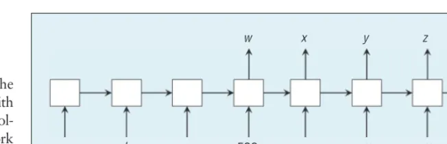
Purely neural machine translation (NMT) is the new MT paradigm. The standard SMT system consists of sev-eral subcomponents that are separately optimized. In contrast, NMT employs only one neural network that’s trained to maximize the conditional likelihood on the bilingual training data. The basic architecture includes two networks: one encodes the variable-length source sen-tence into a real-valued vector, and the other decodes the vector into a variable-length target sentence.
Kyunghyun Cho and colleagues,28
Ilya Sutskever and colleagues,29 and
Dzmitry Bahdanau and colleagues30
fol-low the similar RecurrentNN encoder-decoder architecture (see Figure 9). Given a source sentence in vector
sequence X= (x1, ..., xT), the encoder applies RecurrentNN to obtain a vec-tor C=q(h1, ..., hT) in which ht (1 ≤ ht ≤ T) is calculated as follows:
ht=f(ht−1, xt), (16) where f and q are nonlinear func-tions. Sutskever and colleagues sim-plified the vector to be a fixed-length vector C=q(h1, ..., hT) =hT, whereas Bahdanau and colleagues directly applied the variable-length vector (h1, ..., hT) when predicting each tar-get word.
The decoder also applies Recur-rentNN to predict the target sentence Y= (y1, ..., yT’), where T′ usually dif-fers from T. Each target word yt de-pends on the source context C and all the predicted target words {y1, ..., yt−1}; the probability of Y will be
p Y p yt y yt Ct t
T
( )
=(
{
−}
)
= ′
∑
| 1, , 1 ,1
… . (17)
Sutskever and colleagues chose Ct = C = hT, and Bahdanau and colleagues set Ct=
∑
Tj=1αtj jh.All the network parameters are trained to maximize ∏p(Y) in the bilingual train-ing data. For a specific network struc-ture, Sutskever and colleagues employed deep LSTM to calculate each hidden state, whereas Bahdanau and colleagues applied bidirectional RecurrentNN to compute the source-side hidden-state hj. Both report similar or superior perfor-mance in English-to-French translation compared to the standard phrase-based SMT system.
The MT network architecture is simple, but it has many shortcomings. For example, it restricts tens of thou-sands of vocabulary words for both languages to make it workable in real applications, meaning that many un-known words appear. Furthermore, this architecture can’t make use of the target large-scale monolingual data. Recently, Minh-Thang Luong and colleagues31 and Sebastien Jean
and colleagues32 attempted to solve
the vocabulary problem, but their ap-proaches are heuristic. For example, they used a dictionary in the post-processor to translate the unknown words.
Discussion and Future Directions
Applying DNNs to MT is a hot re-search topic. Indirect application is a relatively conservative attempt be-cause it retains the standard SMT sys-tem’s strength, and the log-linear SMT model facilitates the integration of DNN-based translation features that can employ different kinds of DNNs to deal with different tasks. However, indirect application makes the SMT system much more complicated.
In contrast, direct application is simple in terms of model architecture: a network encodes the source sentence and another network decodes to the target sentence. Translation quality is improving, but this new MT architec-ture is far from perfect. There’s still an open question of how to efficiently cover most of the vocabulary, how to make use of the target large-scale
Figure 9. Neural machine translation (NMT) architecture. The model reads a source sentence abc and produces a target sentence wxyz.
N A T U R A L L A N G U A G E P R O C E S S I N G
monolingual data, and how to utilize more syntactic/semantic knowledge in addition to source sentences.
For both direct and indirect appli-cations, DNNs boost translation per-formance. Naturally, we’re interested in the following questions:
• Why can DNNs improve transla-tion quality?
• Can DNNs lead to a big break- through?
• What aspects should DNNs im-prove if they’re to become an MT panacea?
For the first question, DNNs rep-resent and operate language units in the continuous vector space that fa-cilitates the computation of semantic distance. For example, several algo-rithms such as Euclidean distance and cosine distance can be applied to cal-culate the similarity between phrases or sentences. But they also capture much more contextual information than standard SMT systems, and data sparseness isn’t a big problem. For ex-ample, the RecurrentNN can utilize all the history information before the cur-rently predicted target word; this is im-possible with standard SMT systems.
For the second question, DNNs haven’t achieved huge success with MT until recently. We’ve conducted some analysis and propose some key problems for SMT with DNNs:
• Computational complexity. Be-cause the network structure is com-plicated, and normalization over the entire vocabulary is usually required, DNN training is a time-consuming task. Training a stan-dard SMT system on millions of sentence pairs only requires about two or three days, whereas train-ing a similar NMT system can take several weeks, even with powerful GPUs.
• Error analysis. Because the DNN-based subcomponent (or NMT) deals with variables in the real-valued con-tinuous space and there are no effec-tive approaches to show a meaningful and explainable trace from input to output, it’s difficult to understand why it leads to better translation per-formance or why it fails.
• Remembering and reasoning. For cur-rent DNNs, the continuous vector representation (even using LSTM in RecurrentNN) can’t remember full in-formation for the source sentence. It’s quite difficult to obtain correct target translation by decoding from this rep-resentation. Furthermore, unlike other sequence-to-sequence NLP tasks, MT is a more complicated problem that requires rich reasoning operations (such as coreference resolution). Cur-rent DNNs can’t perform this kind of reasoning with simple vector or ma-trix operations.
T
hese problems tell us thatDNNs have a long way to go in MT. Nevertheless, due to their ef-fective representations of languages, they could be a good solution eventu-ally. To achieve this goal, we should pay attention to the path ahead.
First, DNNs are good at handling continuous variables, but natural lan-guage is composed of abstract discrete symbols. If they completely abandon discrete symbols, DNNs won’t fully control the language generation pro-cess: sentences are discrete, not con-tinuous. Representing and handling both discrete and continuous vari-ables in DNNs is a big challenge.
Second, DNNs represent words, phrases, and sentences in continuous space, but what if they could mine deeper knowledge, such as parts of speech, syntactic parse trees, and knowledge graphs? What about ex-ploring wider knowledge beyond the
sentence, such as paragraphs and dis-course? Unfortunately, representation, computation, and reasoning of such information in DNNs remain a diffi-cult problem.
Third, effectively integrating DNNs into standard SMT is still worth trying. In the multicomponent system, we can study which subcomponent is indis-pensable and which can be completely replaced by DNN-based features. In-stead of the log-linear model, we need a better mathematical model to combine multiple subcomponents.
Fourth, it’s interesting and impera-tive to investigate more efficient algo-rithms for parameter learning of the complicated neural network architec-tures. Moreover, new network archi-tectures can be explored in addition to existing neural networks. We believe that the best network architectures for MT must be equipped with representa-tion, remembering, computarepresenta-tion, and reasoning, simultaneously.
Acknowledgments
This research work was partially funded by the Natural Science Foundation of China un-der grant numbers 61333018 and 61303181, the International Science and Technology Cooperation Program of China under grant number 2014DFA11350, and the High New Technology Research and Development Pro-gram of Xinjiang Uyghur Autonomous Re-gion, grant number 201312103.
References
1. Y. Bengio et al., “A Neural Probabilistic Language Model,” J. Machine Learning Research, vol. 3, 2003, pp. 1137–1155; www.jmlr.org/papers/volume3/bengio03a/ bengio03a.pdf.
2. J.L. Elman, “Distributed Representations, Simple Recurrent Networks, and Gram-matical Structure,” Machine Learning, vol. 7, 1991, pp. 195–225; http://crl.ucsd. edu/~elman/Papers/machine.learning.pdf. 3. R. Socher et al., “Semi-supervised
and Natural Language Process, 2011; http://nlp.stanford.edu/pubs/SocherPen-ningtonHuangNgManning_EMNLP2011. pdf.
4. J.B. Pollack, “Recursive Distributed Representations,” Artificial Intelligence, vol. 46, no. 1, 1990, pp. 77–105. 5. Y. LeCun et al., “Gradient-Based
Learn-ing Applied to Document Recognition,” Proc. IEEE, vol. 86, no. 11, 1998, pp. 2278–2324.
6. F.J. Och and H. Ney, “Discriminative Training and Maximum Entropy Mod-els for Statistical Machine Translation,” Proc. ACL, 2002, pp. 295–302. 7. D. Xiong, Q. Liu, and S. Lin,
“Maxi-mum Entropy Based Phrase Reordering Model for Statistical Machine Transla-tion,” Proc. ACL, 2006, pp. 521–528. 8. N. Yang et al., “Word Alignment
Model-ing with Context Dependent Deep Neural Network,” Proc. ACL, 2013, pp. 41–46. 9. A. Tamura, T. Watanabe, and E.
Sumita, “Recurrent Neural Networks for Word Alignment Model,” to be published in Proc. ACL, 2015. 10. W.Y. Zou et al., “Bilingual Word
Embed-dings for Phrase-Based Machine Transla-tion,” Proc. Empirical Methods and Natural Language Process, 2013, pp. 1393–1398.
11. J. Gao et al., “Learning Continuous Phrase Representations for Translation Modeling,” Proc. ACL, 2014; www. aclweb.org/anthology/P14-1066.pdf. 12. J. Zhang et al., “Bilingually-Constrained
Phrase Embeddings for Machine Transla-tion,” Proc. ACL, 2014, pp. 111–121. 13. L. Cui et al., “Learning Topic
Represen-tation for SMT with Neural Networks,” Proc. ACL, 2014; http://aclweb.org/ anthology/P/P14/P14-1000.pdf. 14. P. Li, Y. Liu, and M. Sun, “Recursive
Au-toencoders for ITG-Based Translation,” Proc. Empirical Methods and Natural Language Process, 2013, pp. 151–161. 15. P. Li et al., “A Neural Reordering
Model for Phrase-Based Translation,” Proc. Conf. Computational Linguistics (COLING), 2014, pp. 1897–1907.
16. F. Zhai et al., “RNN-Based Derivation Structure Prediction for SMT,” Proc. ACL, 2014, pp. 779–784.
17. J. Zhang et al., “Mind the Gap: Machine Translation by Minimizing the Semantic Gap in Embedding Space,” Proc. AAAI, 2014, pp. 1657–1664.
18. S. Liu et al., “A Recursive Recurrent Neu-ral Network for Statistical Machine Trans-lation,” Proc. ACL, 2014, pp. 1491–1500. 19. A. Vaswani et al., “Decoding with
Large-Scale Neural Language Models Improves Translation,” Proc. Empirical Methods and Natural Language Process, 2013; https:// aclweb.org/anthology/D/D13/D13-1.pdf. 20. T. Mikolov, “Statistical Language
Models Based on Neural Networks,” presentation at Google, 2012; www.fit. vutbr.cz/~imikolov/rnnlm/google.pdf. 21. M. Auli and J. Gao, “Decoder Integration
and Expected BLEU Training for Recurrent Neural Network Language Models,” Proc. ACL, 2014; http://research.microsoft.com/ pubs/217163/acl2014_expbleu_rnn.pdf. 22. Y. Hu et al., “Minimum Translation
Modeling with Recurrent Neural Net-works,” Proc. European ACL, 2014; www.cs.umd.edu/~ynhu/publications/ eacl2014_rnn_mtu.pdf.
23. Y. Wu, T. Watanabe, and C. Hori, “Re-current Neural Network-Based Tuple Se-quence Model for Machine Translation,” Proc. Conf. Computational Linguistics (COLING), 2014; http://anthology. aclweb.org/C/C14/C14-1180.pdf. 24. M. Auli et al., “Joint Language and
Translation Modeling with Recurrent Neural Networks,” Proc. Empirical Methods and Natural Language Process,
2013; http://research.microsoft.com/ pubs/201107/emnlp2013rnnmt.pdf. 25. J. Devlin et al., “Fast and Robust Neural
Network Joint Models for Statistical Ma-chine Translation,” Proc. ACL, 2014; http:// aclweb.org/anthology/P/P14/P14-1000.pdf. 26. F. Meng, “Encoding Source Language
with Convolutional Neural Network for Machine Translation,” arXiv preprint arXiv:1503.01838, 2015.
27. J. Zhang, D. Zhang, and J. Hao, “Local Translation Prediction with Global Sen-tence Representation,” to be published in Proc. Int’l J. Conf. Artificial Intelligence, 2015.
28. K. Cho et al., “Learning Phrase Represen-tations Using RNN Encoder-Decoder for Statistical Machine Translation,” Proc. Empirical Methods and Natural Lan-guage Processing, 2014, pp. 355–362. 29. I. Sutskever, O. Vinyals, and Q.V. Le,
“Sequence to Sequence Learning with Neural Networks,” Proc. Neural In-formation Processing Systems (NIPS), 2014; http://papers.nips.cc/paper/5346- sequence-to-sequence-learning-with-neural-networks.pdf.
30. D. Bahdanau, K. Cho, and Y. Bengio, “Neural Machine Translation by Jointly Learning to Align and Translate,” arXiv preprint arXiv:1409.0473, 2014. 31. T. Luong et al., “Addressing the Rare
Word Problem in Neural Machine Translation,” arXiv preprint arX-iv:1410.8206, 2014.
32. S. Jean et al., “On Using Very Large Target Vocabulary for Neural Machine Translation,” arXiv preprint arX-iv:1412.2007, 2014.
tion at the Institute of Automation, Chinese Academy of Sciences. His research interests include machine translation, multilingual natural language processing, and statistical learning. Zhang has a PhD in computer science from the Institute of Automation, Chi-nese Academy of Sciences. Contact him at [email protected].