A multiwavelet approach to the direct so

FYS-3900

Master’s Thesis

in Physics

A multiwavelet approach to the direct

solution of the Poisson equation:

implementation and optimization

Stig Rune Jensen

November, 2009

Faculty of Science and Technology

Department of Physics and Technology

FYS-3900

Master’s Thesis

in Physics

A multiwavelet approach to the direct

solution of the Poisson equation:

implementation and optimization

Stig Rune Jensen

Contents

1 Introduction 2

I

Theory

6

2 The multiwavelet basis 8

2.1 Orthogonal MRA . . . 8

2.2 Multiwavelets . . . 9

2.3 The wavelet basis . . . 10

2.4 The scaling basis . . . 11

2.5 Multiwavelets inddimensions . . . 13

3 Function representation 16 3.1 Function projection . . . 16

3.2 Multiresolution functions . . . 16

3.3 Multiresolution functions inddimensions . . . 18

3.4 Addition of functions . . . 19

3.5 Multiplication of functions . . . 20

4 Operator representation 24 4.1 Operator projection . . . 24

4.2 Multiresolution operators . . . 25

4.3 Integral operators . . . 29

4.4 The Poisson operator . . . 30

II

Implementation

32

5 The MRChem program 34 5.1 Data structures . . . 34

5.2 Adaptive algorithm . . . 35

5.3 Function projection . . . 36

5.4 Addition of functions . . . 38

5.5 Multiplication of functions . . . 39

6 Results 46

6.1 Function projection . . . 46

6.2 Addition of functions . . . 50

6.3 Multiplication of functions . . . 53

6.4 Operator application . . . 55

6.5 Nuclear potential . . . 56

6.6 Electronic potential . . . 60

6.7 Optimization . . . 61

Acknowledgements

First of all I would like to thank my real supervisor, Ass. Prof. Luca Frediani for all help during the last two years, and for introducing me to the facinating theory of multiwavelets. I would also like to thank myformal supervisor Prof. Inge Røeggen, for letting me drift off to the Chemistry Department to write my thesis.

I would like to use the opportunity to thank the Department of Chemistry at the University of Tromsø for the generous financial contribution for my trip to the European Summershool of Computational Chemistry in the fall of 2009. I would also like to thank the CTCC for their financial support for various sem-inars and group meetings during my time as a master student, as well as for their contribution to the above mentioned summer school.

Chapter 1

Introduction

The work of this thesis has been contributing in the development of the program package MRChem, which is a code developed at the University of Tromsø [1] that is aiming at a fully numerical treatment of molecular systems, based on Density Functional Theory (DFT). There are currently a huge number of these program packages available, each with more or less distinct features, and what separates MRChem from all of these is the choice of basis functions. While traditional computational chemistry programs use Gaussian type basis sets for their efficient evaluation of two- and four-electron integrals, MRChem is based on the multiresolution wavelet basis.

Wavelet theory is a rather young field of mathematics, first appearing in the late 1980s. The initial application was in signal theory [2] but in the early 90s, wavelet-based methods started to appear for the solution of PDEs and inte-gral equations [3][4], and in recent years for application in electronic structure calculations [5][6][7].

The Kohn-Sham equations

In the Kohn-Sham [8] formulation of DFT the eigenvalue equations for the electronic structure can be written

[−1₂∇2+Vef f(r)]ψi(r) =ǫiψi(r) (1.1)

where the effective potential is the collection of three terms

Vef f(r) =Vext(r) +Vcoul(r) +Vxc (1.2)

where the external potentialVextis usually just the electron-nuclear attraction, the Coulomb potential Vcoul is the electron-electron repulsion and Vxc is the exchange-correlation potential which (in principle) includes all non-classical ef-fects. The functional form ofVxc is not known.

The nuclear charge distribution is a collection of point charges, and the nuclear potential has the analytical form

Vnuc(r) =−

Nnuc

X

α=1 Zα

The electronic charge distribution is given by the Kohn-Sham orbitals

ρ(r) = 2

Ne/2

X

i=1

|ψi(r)|2 (1.4)

assuming a closed shell system with double occupancy. The electronic potential is now given as the solution of the Poisson equation

∇2Vcoul(r) = 4πρ(r) (1.5)

where the orbital-dependence of the potential makes eq.(1.1) a set of non-linear equations that is usually solved self-consistently. The current work will not be concerned with the solution of the Kohn-Sham equations, but is rather a precursor to this where some building blocks required for the DFT calculations are prepared, in particular the solution of the Poisson equation.

The Poisson equation

Solving the Poisson equation for an arbitrary charge distribution is a non-trivial task, and is of major importance in many fields of science, especially in the field of computational chemistry. A huge effort has been put into making efficient Poisson solvers, and usual real-space approaches includes finite difference (FD) and finite element (FE) methods. FD is a a grid-based method, which is solving the equations iteratively on a discrete grid of pointvalues, while FE is expanding the solution in a basis set, usually by dividing space into cubic cells and allocate a polynomial basis to each cell.

It is a well-known fact that the electronic density in molecular systems is rapidly varying in the vicinity of the atomic nuclei, and a usual problem with real-space methods is that an accurate treatment of the system requires high resolution of gridpoints (FD) or cells (FE) in the nuclear regions. Keeping this high resolution uniformly througout space would yield unnecessary high accuracy in the inter-atomic regions, and the solution of the Poisson equation for molecular systems is demanding amultiresolution framework in order to achieve numerical efficiency.

There are ways of resolving these issues using multigrid techniques, and a nice overview of these methods is given by Beck [9], but this thesis is concerned with a third way of doing real-space calculations, one where the multiresolution character is inherent in the theory, namely using wavelet bases.

Part I

Chapter 2

The multiwavelet basis

A suitable gateway to the theory of multiwavelets is through the idea of mul-tiresolution analysis (MRA). A detailed description of MRAs can be found in Keinert [10], from which a brief summary of the key issues are given in the fol-lowing. This work is concerned with orthogonal MRA only, and for a description of the general bi-orthogonal MRA the reader is referred to Keinerts book.

2.1

Orthogonal MRA

A multiresolution analysis is an infinite nested sequence of subspaces ofL2_(R)

V0

k ⊂Vk1⊂ · · · ⊂Vkn⊂ · · · (2.1)

with the following properties

1. V∞

k is dense in L2

2. f(x)∈Vn

k ⇐⇒f(2x)∈Vkn+1 , 0≤n≤ ∞

3. f(x)∈Vn

k ⇐⇒f(x−2−nl)∈Vkn , 0≤l≤(2n−1)

4. There exists a function vector φof lengthk+ 1 inL2such that

{φj(x) : 0≤j≤k}

forms a basis forV0 k.

This means that if we can construct a basis ofV0

k, which consists of onlyk+ 1

functions, we can construct a basis of any space Vn

k , by simple compression

(by a factor of 2n_{), and translations (to all dyadic grid points at scale n), of}

the originalk+ 1 functions, and by increasing the scalen, we are approaching a complete basis of L2_{. Since V}n

k ⊂ V n+1

k the basis functions of Vkn can be

expanded in the basis ofV_kn+1

φnl(x) def

= 2n/2φ(2nx−l) =X

l

H(l)φn+1l (x) (2.2)

where the H(l)_{s are the so-called filter matrices that describes the}

The MRA is called orthogonal if

hφn₀(x),φn_l(x)i=δ0lIk+1 (2.3) where Ik+1 is the (k+ 1)×(k+ 1) unit matrix, andk+ 1 is the length of the function vector. This orthogonality condition means that the functions are or-thogonal both within one function vector and through all possible translations on one scale, butnot through the different scales.

Complementary to the nested sequence of subspacesVn

k, we can define another

series of spacesWn

k that complementsVkn in V n+1 k

V_kn+1=Vkn⊕Wkn (2.4)

where there exists another function vector ψ of lenght k+ 1 that, with all its translations on scale n forms a basis for Wn

k. Analogously to eq.(2.2) the

function vector can be expanded in the basis ofV_kn+1

ψn_l(x)def= 2n/2ψ(2nx−l) =X

l

G(l)φn+1_l (x) (2.5)

with filter matrices G(l)_{. In orthogonal MRA the functions ψ fulfill the same}

othogonality condition as eq.(2.3), and if we combine eq.(2.1) and eq. (2.4) we see that they must also be orthogonal with respect to different scales. Using eq.(2.4) recursively we obtain

Vkn=Vk0⊕Wk0⊕Wk1⊕ · · · ⊕Wkn−1 (2.6)

which will prove to be an important relation.

2.2

Multiwavelets

There are many ways to choose the basis functionsφand ψ (which define the spanned spacesVn

k and Wkn), and there have been constructed functions with

a variety of properties, and we should choose the wavelet family that best suits the needs of the problem we are trying to solve. Otherwise, we could start from scratch and construct a new family, one that is custom-made for the problem at hand. Of course, this is not a trivial task, and it might prove more efficient to use an existing family, even though its properties are not right on cue.

There is a one-to-one correspondence between the basis functions φ and ψ, and the filter matrices H(l) _{and G}(l) _{used in the two-scale relation equations}

eq. (2.2) and eq.(2.5), and most well known wavelet families are defined only by their filter coefficients. This usually leads to non-smooth functions, like the DaubechiesD2 wavelet family (figure 2.1).

In the following we are taking a different, more intuitive approach, which follows the original construction of multiwavelets done by Alpert [4]. We define the

scaling space Vn

k as the space of piecewise polynomial functions

Vn k

def

= {f : all polynomials of degree ≤ k on the interval(2−n_l,2−n_{(l+ 1))} f or0≤l <2n_{, f vanishes elsewhere}}

Figure 2.1: DaubechiesD2 scaling (left) and wavelet (right) function.

It is quite obviuos that one polynomial of degree kon the interval [0,1] can be exactly reproduced by two polynomials of degree k, one on the interval [0,1

2]

and the other on the interval [1

2,1]. The spacesV n

k hence fulfills the MRA

con-dition eq.(2.1), and if the polynomial basis is chosen to be orthogonal, the Vn k

constitutes an orthogonal MRA.

2.3

The wavelet basis

The wavelet space Wn

k is defined, according to eq. (2.4), as the orthogonal

complement of Vn k inV

n+1

k . The multiwavelet basis functions ofWkn are hence

piece-wise polynomials of degree≤koneach of the two intervals on scale n+1 that overlaps withoneinterval on scale n. These piece-wise polynomials are then made orthogonal to a basis of Vn

k and to each other. The construction of the

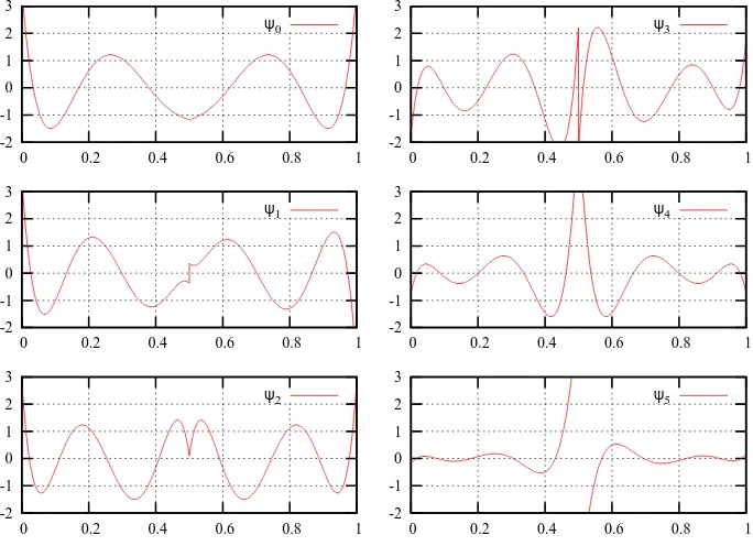
multiwavelet basis follows exactly [4] where a simple Gram-Schmidt orthogono-lization were employed to construct a basis that met the necessary orthogonality conditions. The wavelet functions for k= 5 are shown in figure 2.2

One important property of the wavelet basis is the number of vanishing mo-ments. The k-th continuous moment of a functionψis defined as the integral

µk def=

Z 1

0

xk_{ψ(x)dx (2.8)}

and the function ψhasM vanishing moments if

µk = 0, k= 0, . . . , M−1

The vanishing moments of the wavelet functions gives information on the ap-proximation order of the scaling functions. If the wavelet function ψ has M

vanishing moments, any polynomial of order≤M−1 can be exactly reproduced by the scaling functionφ, and the error in representing an arbitrary function in the scaling basis is of M-th order. By construction, xi _{is in the spaceV}0

k for

0≤i≤k, and sinceW0

-2

Figure 2.2: First six wavelet functions at scale zero

2.4

The scaling basis

The construction of the scaling functions is quite straightforward; k+ 1 suit-able polynomials are chosen to span any polynomial of degree≤kon the unit interval. The total basis for Vn

k is then obtained by appropriate dilation and

translation of these functions. Of course, any polynomial basis can be used, the simplest of them the standard basis {1, x, . . . , xk_{}. However, this basis is}

not orthogonal on the unit interval and cannot be used inorthogonal MRA. In the following, two choices of orthogonal scaling functions will be presented, and even though they span exactly the same spaces Vn

k there are some important

numerical differences between the two. These differences will be considered in the implementation part of this thesis.

In order to construct a set of orthogonal polynomials we could proceed in the same manner as for the wavelet functions and do a Gram-Schmidt orthogo-nalization of the standard basis {1, x, . . . , xk_{}. If this is done on the interval} x∈[−1,1] we end up with the Legendre polynomials{Lj}k

j=0. These functions

are usually normalized such that Lj(1) = 1 for all j. To make the Legendre scaling functions φL

j we transform the Legendre polynomials to the interval x∈[0,1], andL2_-normalize

φLj(x) =

p

2j+ 1Lj(2x−1), x∈[0,1] (2.9)

The basis for the spaceVn

k is then made by proper dilation and translation of φL

-2

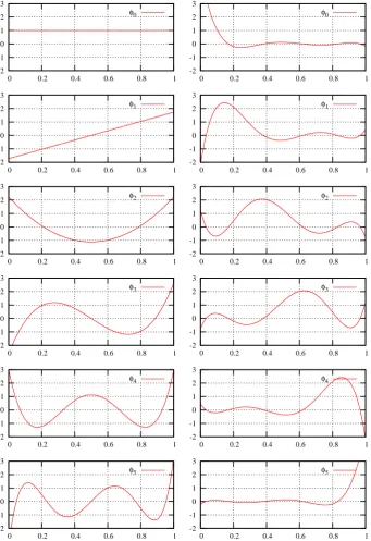
Alpert et al. [11] presented an alternative set of scaling functions with inter-polating properties. These Interpolating scaling functions φI

j are based on the

Legendre scaling functions{φL

j}kj=0, and the roots{yj}kj=0and weights{wj}kj=0

of the Gauss-Legendre quadrature of orderk+ 1, and are organized in the linear combinations

φIj(x) =√wj kp

X

i=0

φLi(yj)φLi(x), x∈[0,1] (2.10)

Again the basis ofVn

k is made by dilation and translation ofφIj. The Legendre

and Interpolating scaling functions of orderk= 5 are shown in figure2.3. The construction ofφI

j gives them the interpolating property

φIj(yi) = δji

√_wi (2.11)

which will prove important for numerical efficiency.

A detailed discussion on the properties of Interpolating wavelets can be found in Donoho [12], but the case of Interpolating multiwavelets is somewhat differ-ent. An important property of Interpolating wavelets is thesmoothness of any function represented in this basis. This property stems from general Lagrange interpolation. In the multiwavelet case the interpolating property applieswithin

one scaling function vector only, which means that functions represented in this basis can be discontinous in any merging point between the different transla-tions on any scale. This is also the case for the Legendre scaling functransla-tions, and it makes differentiation awkward in these bases.

With the basis functions in place we can now use these to construct the filter matrices that fulfill the two-scale conditions eq.(2.2) and eq.(2.5). The details of this construction are given in Alpert et al. [11], and will not be presented here, but we specifically end up with four matrices H(0)_{, H}(1)_{, G}(0) _{and G}(1)_,

which size and contents are dependent on the order and type of scaling functions chosen. Eq.(2.2) and eq.(2.5) thus reduces to

φn_l =H(0)φn+1_2l +H(1)φn+1_2l+1

ψnl =G(0)φn+12l +G (1)

φn+1_2l+1 (2.12)

2.5

Multiwavelets in

d

_dimensions

When dealing with multidimensional multiwavelets we open a notational can of worms that easily gets confusing. The following notation is aiming to be as intuitive as possible, and is similar to the one presented in [1].

Multidimensional wavelets are usually constructed by tensor products, where the scaling space is defined as

Vkn,d def

=

d

O

The basis for this d-dimensional space is given as tensor products of the one-dimensional bases.

Φnj,l(x) = Φnj1j2...jd,l1l2...ld(x1, x2, . . . , xd)

def

=

d

Y

i=1

φnji,li(xi) (2.14)

The number of basis functions on each hypercube l = (l1, l2, . . . , ld) becomes (k+ 1)d, while the number of such hypercubes on scale nbecomes 2dn, which again means that the total number of basis functions is growing exponentially with the number of dimensions.

The wavelet space can be defined using eq.(2.4)

V_kn+1,d=

d

O

V_kn+1=

d

O

(Vkn⊕Wkn) (2.15)

where the pure scaling term obtained when expanding the product on the right hand side of eq.(2.15) is recognized as V_kn,d, making the wavelet space W_kn,d

consist of all the remaining terms of the product, which are terms that contain at least one wavelet space.

To achieve a uniform notation, we can introduce a ”generalized” one-dimensional wavelet function{ϕα,n_j,l }that, depending on the indexαcan be either the scaling or the wavelet function

ϕαi,n

ji,li

def

=

_φn

ji,li ifαi= 0

ψn

ji,li ifαi= 1

(2.16)

The wavelet functions for thed-dimensional space can thus be expressed as

Ψα,nj,l(x) =

d

Y

i=1 ϕαi,n

ji,li(xi) (2.17)

Where the totalαindex on Ψ separates the 2d_{different possibilities of combining}

scaling/wavelet functions with the same index combination j= (j0, j1, . . . , jk).

αis given by the binary expansion

α=

d

X

i=1

2i−1αi (2.18)

and thus runs from 0 to 2d_{−1. By closer inspection we see thatα= 0 recovers}

the pure scaling function

Ψ0,n_j,l(x)≡Φn

j,l(x) (2.19)

and we will keep the notation Φn

j,l for the scaling function, and exclude the

α= 0 term in the wavelet notation when treating multidimensional functions.

We can immediately see that the dimensionality of the wavelet space is higher than the scaling space on the same scalen, specifically 2d_{−1 times higher. This}

must be the case in order to conserve the dimensionality through the equation

sincedim(V_kn+1,d) = 2d_dim(Vn,d k ).

As for the monodimensional case we can define filter matrices that transform the scaling functions at scalen+1,{Φn+1_j,l }, into scaling and wavelet functions at scalen,{Ψα,n_j,l}2α=0d−1. Details of this construction can be found in [1], where the

Chapter 3

Function representation

With the multiwavelet basis introduced, we have a hierarchy of basis sets with increasing flexibility, and we can start making approximations of functions by expanding them in these bases.

3.1

Function projection

We introduce the projection operator Pn _{that projects an arbitrary function} f(x) onto the basis{φn

j,l}of the scaling spaceVn (in the remaining of this text

the subscript k of the scaling and wavelet spaces will be omitted, and it will always be assumed that we are dealing with a k-order polynomial basis).

f(x)≈Pnf(x)def= fn(x) =

2n−1

X

l=0 k

X

j=0

sn,f_j,l φnj,l(x) (3.1)

where the expansion coefficients sn,f_j,l , the so-calledscaling coefficients, are ob-tained by the usual integral

sn,fj,l def

= hf, φnj,li=

Z 1

0

f(x)φnj,l(x)dx (3.2)

If this approximation turns out to be too crude, we double our basis set by increasing the scale and perform the projection Pn+1_{. This can be continued}

until we reach a scaleN where we are satisfied with the overall accuracy offN

relative to the true functionf.

3.2

Multiresolution functions

We can also introduce the projection operatorQn _{that projectsf(x) onto the}

wavelet basis of the spaceWn

Qnf(x)def= dfn(x) =

2n₋₁

X

l=0 k

X

j=0

where thewavelet coefficients are given as

dn,f_j,l def=hf, ψnj,li=

Z 1

0

f(x)ψj,ln(x)dx (3.4)

According to eq.(2.4) we have the following relationship between the projection operators

Pn+1_=Pn_+Qn _(3.5)

and it should be noted thatdfn _{is not an approximation of f, but rather the}

difference between two approximations. We know that the basis ofV∞ _{forms a} complete set inL2_{, which implies thatP}∞_{must be the identity operator.} Com-bining this with eq.(3.5) we can decompose the functionf into multiresolution contributions

This expansion is exact, but contains infinitely many coefficients. If we want to make approximations of the functionf we must truncate the infinite sum in the wavelet expansion at some finest scaleN

f(x)≈fN(x) =

This expansion is completely equivalent to eq.(3.1) (withn=N) both in terms of accuracy and in number of expansion coefficients. However, as we have seen, the wavelet projectionsdfn _{are defined as the difference between two}

consecu-tive scaling projections, and since we know, for L2 _{functions, that the scaling}

projections is approaching the exact functionf, we also know that thewavelet

projections must approach zero. This means that as we increase the accuracy by increasingN in eq.(3.7) we know that the wavelet terms we are introducing will become smaller and smaller, and we can choose to keep only the terms that are above some threshold. This makes the multiresolution representation preferred since it allows for strict error control with a minimum of expansion coefficients. This is the heart of wavelet theory.

Wavelet transforms

The filter matrices H(0), H(1), G(0) and G(1) allow us to change between the representations eq.(3.1) and eq.(3.7). The two-scale relations of the scaling and wavelet functions eq.(2.12) apply directly to the scaling coefficient vectors sn_l, and wavelet coefficient vectorsdnl, and the coefficients on scalenare obtained

by the coefficients on scalen+ 1 through

This transformation is called forward wavelet transform or wavelet decompo-sition of the scaling coefficients on scale n+ 1. By doing this decomposition recursively we can get from eq.(3.1) to eq.(3.7). Rearranging eq.(3.8) we arrive at the backward wavelet transform or wavelet reconstruction

sn+1_2l =H(0)Tsn_l +G(0)Tdn_l

sn+1_2l+1=H(1)Tsnl +G(1)Tdnl

(3.9)

where the transposed filter matrices are used.

It should be emphasized that these wavelet transforms do not change the func-tionthat is represented by these coefficients, they just change thebasis set used to represent the exact same function. This means that the accuracy of the rep-resentation is determined only by the finest scale of which the coefficients were obtained byprojection, and a backward wavelet transform beyond this scale will not improve our approximation (but it will increase the number of expansion coefficients).

The true power of multiwavelets is that, by truncating eq.(3.7)locally whenever the wavelet coefficients are sufficiently small, we end up with a space adaptive basis expansion, in that we are focusing the basis functions in the regions of space where they are most needed.

3.3

Multiresolution functions in

d

_dimensions

The multidimensional function representation is obtained similarly to eq.(3.1) by projection onto the multidimensional basis eq.(2.14)

f(x)≈fn(x) =X

l

X

j

sn,fj,lΦ

n

j,l(x) (3.10)

where the sums are over all possible translation vectors l = (l1, . . . , ld) for 0≤li ≤2n_{−1, and all possible scaling function combinationsj = (j1, . . . , jd)}

for 0 ≤ji ≤k. The scaling coefficients are obtained by the multidimensional integral

sn,f_j,l def=hf,Φn

j,li=

Z

[0,1]d

f(x)Φn

j,l(x)dx (3.11)

The wavelet components are given as

dfn(x) =X

l

X

j

2d₋₁

X

α=1

dα,n,fj,l Ψ

α,n

j,l (x) (3.12)

where thelandjsummations are the same as in eq.(3.10), and theαsum is over all combinations of scaling/wavelet functions (excluding the pure scalingα= 0). The expansion coefficients are obtained by the multidimensional projection

dα,n,f_j,l def= hf,Ψα,n_j,li=

Z

[0,1]d

We can express a multidimensional functionf(x) by its multiresolution contri-butions as for the monodimensional case

fN(x) =X

j

s0,fj,0Φ

0

j,0(x) +

N−1

X

n=0

X

l

X

j

2d₋₁

X

α=1

dα,n,fj,l Ψ

α,n

j,l (x) (3.14)

Wavelet transforms in

d

_dimensions

Thed-dimensional filter matrices were obtained by tensor products of the monodi-mensional filters. This means that by the tensor structure of the multidimen-sional basis, we can perform the wavelet transform one dimension at the time. This allows for the situation where the basis is represented at different scales in different directions. Specifically, in two dimensions, the way to go from the scaling plus wavelet representation on the squarelat scalento the pure scaling representation in the four subsquares oflat scalen+ 1, we perform the trans-form first in one direction by dividing the square into two rectangular boxes, and then the other direction, dividing the two rectangels into four squares.

One important implication of this tensor structure is that the work done in the

d-dimensional transform scales linearly in the number of dimensions. If the full

d-dimensional filter matrix had been applied, the work would have scaled as the power of the dimension, hence limiting the practical use in higher dimensions. A more rigorous treatment of the multidimensional wavelet transforms can be found in [13].

3.4

Addition of functions

The addition of functions in the multiwavelet basis is quite straightforward, since it is represented by the mappings

Vn+Vn→Vn

Wn+Wn→Wn (3.15)

This basically means that the projection of the sum equals the sum of the pro-jections. In the polynomial basis this is simply the fact that the sum of two

k-order polynomials is still ak-order polynomial.

Consider the equation h(x) =f(x) +g(x). Projectinghonto the scaling space yields

hn(x) =Pnh(x)

=Pn(f(x) +g(x)) =Pnf(x) +Png(x)

=fn(x) +gn(x) (3.16)

and similarly

The functions f(x) and g(x) are expanded in the same basis set and the sum simplifies to an addition of coefficients belonging to the same basis function and can be done one scale at the time.

hn(x) =fn(x) +gn(x)

The generalization to multiple dimensions is trivial, and will not be discussed at this point.

3.5

Multiplication of functions

Multiplication of functions in the multiwavelet basis is somewhat more involved than addition. The reason for this is that, in contrast to eq.(3.15), the product is represented by the mapping [14]

Vn

k ×Vkn→V2kn (3.20)

This means that the product of two functions falls outside of the MRA and needs to be projected back onto the scaling space sequence. This is easily seen in our polynomial basis; the product of two piecewise degree≤kpolynomials is a piecewise polynomial of degree≤2k, which cannot be exactly reproduced by any piecewise degree≤kpolynomial (other than in the limitV∞_{). In particular} this means that the product of two functions on a given scale ”spills over” into the finer scales, in the sense that

Vn×Vn→Vn⊕ ∞

M

n′=n

Wn′ (3.21)

Working with a finite precision it is desirable to make the product as accurate as each of the multiplicands. This is done by terminating the sum in eq.(3.21) at a sufficiently large scaleN.

Vn×Vn →Vn⊕

N−1

M

n′=n

Wn′ =VN (3.22)

Assume now thatnis the finest scale present in either of the multiplicands, and

part of this thesis, and in the following it is simply assumed thatN is known a priori. We know that

Vn⊂Vn+1 ⊂ · · · ⊂VN

which means that the multiplication could just as well have been written

VN ×VN →VN

where the representations of the multiplicands on scale N is obtained by a se-ries of backward wavelet transforms. As pointed out before this will result in an increase in the number of coefficients without changing theinformationthat we are able to extract from these functions. Thisoversampling of the multipli-cands allow us to relate the scaling coefficients of the product on scaleN to the coefficiens of the multiplicands on the same scale.

Finally, when we have obtained the scaling coefficients of the product on scaleN

we do a forward wavelet transform to obtain wavelet coefficients on the coarser scales. We can now throw away all wavelet terms that are sufficiently small, and we have an adaptive representation of the product.

Scaling function multiplication

Consider the equation h(x) =f(x)×g(x). We want to represent the function

h(x) at some scaleN

hN(x) =PNh(x)

=PN(f(x)×g(x)) (3.23)

However, as we have seen, the projection of the product eq.(3.23) does not

equal the product of the projections, and we will actually have to perform this projection. We will of course not have available the functions f(x) and g(x) analytically, so the best thing we can do is

hN(x)≈PN fN(x)×gN(x)def

= PN˜h(x) (3.24)

The scaling coefficients of the product is approximated by the projection integral

sN,h_jh_,l ≈

and if the scaleN is chosen properly, the error in the coefficients can be made negligeable compared to the total error inhN_{(x). We see that the multiplication}

is related to a limited number of integrals, specifically (k+ 1)3 _different

Multiplication in

d

_dimensions

The generalization to multiple dimensions is quite straightforward, using the notation of eq.(2.14)

sN,h_jh_,l= 2

NX

jf

X

jg

sN,f_jf_,ls

N,g

jg_,l

Z

[0,1]d

Φ0

jf_,0(x)Φ

0

jg_,0(x)Φ0_jh_,0(x)dx

(3.26)

The only difference consists in the number of integrals, which grows exponen-tially in the number of dimensions. The multidimensional integral can however be decomposed into a product of monodimensional ones

Z

[0,1]d

Φ0

jf_,0(x)Φ

0

jg_,0(x)Φ0_jh_,0(x)dx

=

d

Y

i=1

Z 1

0 φ0_jf

i,0

(xi)φ0_jg i,0(xi)φ

0 jh

i,0(xi)dxi (3.27)

and we have again related all the integrals to the same small set of (k+ 1)3

Chapter 4

Operator representation

When we now have a way of expressing an arbitrary function in terms of the multiwavelet basis, and we have the possibility of doing some basic arithmetic operations with these function representations, the next step should be to be able to apply operators to these functions. Specifically, we want to be able to compute the expansion coefficients of a function g(x), given the coefficients of

f(x) based on the equation

[T f](x) =g(x) (4.1)

4.1

Operator projection

When applying the operator we will only have an approximation of the function

f(x) available

[T Pnf](x) = ˜g(x) (4.2)

and we can only obtain in the projected solution

[Pn_{T P}n_{f](x) =P}n_{˜g(x) (4.3)}

Using the fundamental property of projection operators Pn_Pn_=Pn _{we get}

[PnT PnPnf](x) =Pn˜g(x) (4.4)

We now define the projection of the operatorT on scalenas

T ∼ nTndef= PnT Pn (4.5)

This approximation makes sense since limn→∞Pn = 1. We can now represent the entire operation on scalen

n_Tn_fn_{= ˜g}n _(4.6)

Here we should note the difference between ˜gn _andgn _{in that ˜g}n _{isnot the}

pro-jection of the true functiong, but rather the projection of thetrue T operating on the projected f, and one should be concerned of whether the error|g˜n_−gn_|

is comparable to|g−gn_{|, but it can be shown [1] that this will not be a problem}

4.2

Multiresolution operators

Making use of eq.(4.5) and eq.(3.5) we can decompose the operator into mul-tiresolution contributions

and we simplify the notation with the following definitions, eq.(4.5) is repeated for clearity

By truncating the sum in eq.(4.7) we get a multiresolution representation of the operator with finite precision

T ≈ NTN = 0T0+

where the representations ofT andf on scaleN are obtained by wavelet trans-form from their respective finest scales. This matrix equation describes the entire operation, and provided the scaleN has been chosen properly, the result-ing function g can be represented with the same accuracy as f. An adaptive representation of g is obtained by performing a wavelet decomposition of gN

into its multiresolution components, throwing away all wavelet terms that are sufficiently small.

There is (at least) one problem with this matrix representation; the matrixN_TN

is dense, in the sense that it has generally only non-vanishing entries. This is a numerical problem more that a mathematical one, and will lead to algorithms that scale quadratically in the number of basis functions in the system, and one of the main prospects of wavelet theory is to arrive at fast (linear scaling) algorithms.

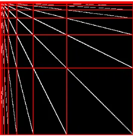
The way to approach this holy grail of numerical mathematics is to realize that the matrices A, B and C will not be dense (at least for the type of operators treated in this work), but rather have a band-like structure where their elements are rapidly decaying away from their diagonals. The reason for this bandedness of the matrices can be found in [3] and will not be discussed here, it suffices to say that it stems from the vanishing moments property of the wavelet functions.

The way to achieve a banded strucure of the operator is thus to decompose it according to eq.(4.9)

N_TN ₌ N−1_TN−1₊ N−1_AN−1₊ N−1_BN−1₊ N−1_CN−1 _(4.11)

The functionsf andg can be decomposed to scaleN−1 by simple filter oper-ations eq.(3.8). According to eq.(4.8)n_Tn _andn_Cn _{produce the scaling part of} g, acting on the scaling and wavelet parts off, respectively. Similarly,n_An _and n_Bn _{produce the wavelet part ofg, by acting on the wavelet and scaling parts}

off, respectively. The matrix equation eq.(4.10) can thus be decomposed as



where the size of the total matrix is unchanged. What has been achieved by this decomposition is a banded structure in three of its four components, leaving only the N−1_TN−1 _{part dense. We can now do the same decomposition of}

and gN−1 _{need to be decomposed as well. To keep everything consistent the} N−1_BN−1 _and N−1_CN−1 _{parts of the operator will have to be transformed}

accoringly. To proceed from here we need the following relations

n_Bn_=Qn_{T P}n

which is the exact change in the operator that is taking place when we decompose

fn _intofn−1_+dfn−1_andgn _intogn−1_+dgn−1_{. The matrix equation will now}

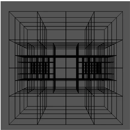
Figure 4.1: Banded structure of the standard operator matrix.

into extremely narrow bandedA-character.

N_TN ₌ 0_T0₊ N−1

X

n=0

n_Cn₊ N−1

X

n=0

n_Bn₊ N−1

X

n=0 n_An

= 0T0+

N−1

X

n=0

0_Cn₊ X

n′_<n

n′

An

!

+

N−1

X

n=0

n_B0₊ X

n′>n n′

An

!

+

N−1

X

n=0 n_An

= 0_T0₊ N−1

X

n=0

0_Cn₊ N−1

X

n=0

n_B0₊ N−1

X

n=0 N−1

X

n′₌₀

n_An′

(4.16)

4.3

Integral operators

We now turn our attention to a specific type of operator; the one-dimensional integral operator given in the form

[T f](x) =

Z

K(x, y)f(y)dy (4.17)

whereKis the two-dimensional operator kernel. The first step is to expand the kernel in the multiwavelet basis

KN(x, y) =X

lx,ly

τN,N_lxly φNlx(x)φ

N

ly(y) (4.18)

where the expansion coefficients are given by the integrals

τnx,ny

Inserting eq.(4.18) into eq.(4.17) yields

N_TN_fN_{(x) =}Z

where the last integral is recognized as the scaling coefficients off

N_TN_fN_{(x) =}X

matrix equation eq.(4.10) written explicitly. As pointed out, the matrixN_TN _is

dense and we would generally have to keep all the terms in eq.(4.21), therefore we want to decompose it to contributions on coarser scales. We introduce the following definitions, eq.(4.19) is repeated for clearity

Equation eq.(4.21) can then be decomposed as

C, respectively, and eq.(4.23) is again the matrix equation eq.(4.12) written explicitly. In this expression the last term involving the α coefficients will be extremely sparse, and this sum can be limited tolx, ly values that differ by less than some predetermined bandwidth |lx−ly| < ΛN−1,N−1_{. The rest of the}

expression eq.(4.23) involves at least one scaling term, so we seek to decompose them further.

The first term in eq.(4.23) can be decomposed in the same manner as eq.(4.21), and the γ andβ terms can be partially decomposed, following the arguments of eq.(4.14) and eq.(4.13), respectively. If we do this all the way to the coarsest scale, we obtain

This is the explicit expression for the standard representation of an operator in the multiwavelet basis eq.(4.16). In eq.(4.24) the majority of terms are included in the last quadruple sum, which is limited to include only terms |lx−ly| <

Λnx,ny_{, making the total evaluation much more efficient than eq.(4.21).}

4.4

The Poisson operator

In order to solve the Poisson equation using the methods described above, we need to rewrite it to an integral form. The equation, in its differential form, is given as

∇2V(x) = 4πρ(x) (4.25)

solu-tion can be written as the integral

V(x) =

Z

G(x,y)ρ(y)dy (4.26)

whereG(x,y) is the Green’s function which is the solution to thefundamental

equation withhomogeneous (Dirichlet) boundary conditions

∇2G(x,y) =δ(x₋y)

G(x,y) = 0 ,x∈boundary (4.27)

This equation can be solved analytically and the Green’s function is given (in three dimensions) simply as

G(x,y) = 1

||x−y|| (4.28)

This is the well known potential arising from a point charge located in the po-sitiony, which is exactly what eq.(4.27) describes.

Numerical separation of the kernel

The Green’s function kernel as it is given in eq.(4.28) is not separable in the cartesian coordinates. However, since we are working with finite precision we can get by with an approximate kernel as long as the error introduced with this approximation is less than our overall accuracy criterion. If we are able to obtain such anumericalseparation of the kernel, the operator can be applied in one direction at the time, allowing us to use the expressions derived above for one-dimensional integral operators to solve the three-dimensional Poisson equa-tion. This is of great importance, not only because we do not have to derive the d-dimensional operator equations, which is at best notationally awkward, but also because it again reduces the scaling behavior to become linear in the dimension of the system.

The Poisson kernel can be made separable by expanding it as a sum of Gaussian functions, specifically

1 ||r−s|| ≈

Mǫ

X

κ=1

aκe−bκ(r−s)2 _(4.29)

where aκand bκ are parameters that needs to be determined, and the number of terms Mǫ, called the separation rank, depends on the accuracy requirement and on what interval this expansion needs to be valid. Details of how to obtain this expansion can be found in [1], and will not be treated here, but it should be mentioned that the separation rank is usually in the order of 100, e.g. it requires

Mǫ = 70 to reproduce 1/r on the interval [10−5_,√_{3] in three dimensions with}

Part II

Chapter 5

The MRChem program

5.1

Data structures

In the following a brief introduction is given to the important data structures that are used in the MRChem program. This will introduce the nomenclature used in the rest of the thesis.

Node

Thenode _{is the multidimensional box on which the set of scaling and wavelet} functions that share the same support are defined. The node_{is specified by its} scalen, which gives its size ([0,2−n_]d_{) and translation vectorl= (l1, l2, . . . , ld),}

which gives its position. The node _{holds the (k+ 1)}d _{scaling coefficients and} (2d_{−1)(k+ 1)}d _{wavelet coefficients that share the same scale and translation.}

It will also keep track of its parent and all 2d _{childrennodes, giving the nodes}

a tree-like structure.

Tree

Thetree_{data structure is basically the multiwavelet representation of a} func-tion. The name originates from the fact that a one-dimensional function is represented as a binary tree of nodes _{(octal tree in three dimesions)} emanat-ing from the semanat-ingle root node _{at scale zero. The}tree _{keeps the entire tree of}

nodes_{, from root to leaf, and each}node _{keeps both the scaling and wavelet}

5.2

Adaptive algorithm

The algorithm used to obtain adaptive representations of functions was pre-sented in [1]. This is a fully on-the-fly algorithm in the sense that one sets out from the coarsest scale and refine the representation scale by scale locally only where it is needed. This in oppose to the originally proposed algorithm where one calculates the uniform representation eq.(3.1) on some finest scale and then do a forward wavelet transform and discards all wavelet terms below some threshold to obtain the adaptive representation eq.(3.7). One obvious ad-vantage of this adaptive algorithm is that we do not need any a priori knowlegde of the global finest scale.

Algorithm 1Generation of adaptive Multiwavelet representation of a function 1: _whilenumber of nodes on current scaleNs>0 _do

2: _foreach node at current scale_do

3: compute scaling and wavelet coefficients

4: if node needs to be refinedthen 5: mark node as non-terminal

6: allocate children nodes

7: update list of nodes at the next scale

8: else

9: mark node as terminal

10: _{end if} 11: _{end for} 12: increment scale

13: _{end while}

The algorithm consists of two loops, the first runs over the ladder of scales, from coarsest to finest, while the second is over thenodes_{present at the current scale.} Once the expansion coeffients of the current node are known, a split check is performed based on the desired precision. If the node _{does not satisfy the} ac-curacy criterion, thenode_{is marked as non-terminal and its children}nodes_are allocated and added to the list of nodes_{needed at the next scale. If the}node does not need to be split, thenode_{is marked as terminal and no children}nodes are allocated. In this way, once the loop overnodes_{on one scale is terminated,} the complete list of nodes _{needed on the next scale has been obtained. Now} the scale counter is incremented and the loop over nodes _{on the next scale is} started. The tree_{is grown until no}nodes _{are needed at the next finer scale.}

There are of course two points in this algorithm that need to be treated fur-ther, the first being the actual computation of the expansion coefficients (line 3). This can be done in one of four ways (projection, addition, multiplication or operator application) and will be treated in the subsequent sections. The second point is how to perform the split check (line 4).

The split check is performed to decide whether or not the function is represented accurately enough on the currentnode_{, based on a predefined relative precision}

ǫ. Formally, this relative precision requires that

where fǫ is our approximation of f. However, this check cannot be performed since the true functionf is generally not known. The check that will be per-formed is based on the fact that the scaling projections will approach the exact function with increasing scale. Consequently, the wavelet projections, which is the difference between two consecutive scaling projections, must approach zero. This means that we can use the norm of the wavelet coefficients on onenode_as a measure for the accuracy of the function represented by thisnode_{, and we will} use the following threshold for the wavelet coefficients on the terminalnodes

||dnl||<2−n/2ǫ||fǫ||2 (5.2)

A justification for this choice of thresholding can be found in [1] and references therein. This algorithm is very general, and as pointed out it can be used to build adaptive representations of functions regardless of how the expansion coefficients are obtained, and in the following sections we will look at four different ways of doing this.

5.3

Function projection

The first step into the multiresolution world will always have to be taken by projection of some analytical function onto the multiwavelet basis. Only then can we start manipulating these representations by additions, multiplications and operators.

Legendre scaling functions

In a perfect world, the projection in eq.(3.2) could be done exactly, and the ac-curacy of the projection would be independent of the choice of polynomial basis. In the real world the projections are done with Gauss-Legendre quadrature and the expansion coefficientssn,fj,l off(x) are obtained as

sn,f_j,l =

Z 2−n(l+1)

2−n_l

f(x)φnj,l(x)dx

= 2−n/2

Z 1

0

f(2−n(x+l))φ0j,0(x)dx

≈ 2−n/2

kq−1

X

q=0

wqf(2−n_(yq+l))φ0

j,0(yq) (5.3)

where {wq}kq−1

q=0 are the weights and {yq} kq−1

q=0 the roots of the Legendre

poly-nomialLkq used inkq-th order quadrature.

By approximating this integral by quadrature we will of course not obtain the exact expansion coefficients. However, it would be nice if we could obtain the

degree≤(k+ 1) when projecting on the basis ofk-order Legendre polynomials, and we will use quadrature orderk+ 1 througout.

In the multidimensional case the expansion coefficients are given by multidi-mensional quadrature

using the following notation for the vector of quadrature roots

yq

def

= (yq1, yq2, . . . , yqd) (5.5)

This quadrature is not very efficient in multiple dimensions since the number of terms scales as (k+ 1)d_{. However, if the functionf is separable and can be}

which is a product of small summations and scales only asd(k+ 1).

The Legendre polynomials show very good convergence forpolynomialfunctions

f(x), and are likely to give more accurate projections. However, most interest-ing functionsf(x) arenot simple polynomials, and the accuracy of the Legendre scaling functions versus a general polynomial basis might not be very different.

Interpolating scaling functions

By choosing the quadrature order to bek+ 1 a very important property of the Interpolating scaling functions emerges, stemming from the specific construction of these functions eq.(2.10), and the use of the k+ 1 order quadrature roots and weights. The interpolating property eq.(2.11) inserts a Kronecker delta whenever the scaling function is evaluated in a quadrature root, which is exactly the case in the quadrature sum. This reduces eq.(5.3) to

sn,f_jl = 2 −n/2

√_wj f(2−n(xj+l)) (5.7)

which obviously makes the projectionk+ 1 times more efficient.

In multiple dimensions this property becomes even more important, since it effectively removes all the nested summations in eq.(5.4) and leaves only one term in the projection

sn,fj,l =f(2

Obtaining the wavelet coefficients

The wavelet coefficients are formally obtained by the projection of the function onto the wavelet basis, and we could derive expressions similar to the scaling expressions based on quadrature. There are however some accuracy issues con-nected to this wavelet quadrature, so we will take another approach that utilizes the wavelet transform. We know that we can obtain the scaling and wavelet co-efficients on scalenby doing a wavelet decomposition of the scaling coefficients on scalen+ 1 according to eq.(3.8). Line 3 of the algorithm is thus performed by computing the scaling coefficients of the 2d children of the currentnode _by the appropriate expression (Legendre or Interpolating), followed by a wavelet decomposition. In this way, wavelet projections are not required.

Quadrature accuracy

We know that by using quadrature in the projection, we are only getting ap-proximate scaling coefficients, and some remarks should be given on this matter. Consider the quadrature performed at scale zero. Ind dimensions this gives a total number of (k+ 1)d _{quadrature points distributed in the unit hypercube}

[0,1]d_{, while the quadrature on scale one will give (k+ 1)}d_{quadrature points on}

each of the 2d _{children cubes contained in the same unit hypercube. This will}

obviousy increase the accuracy of the quadrature, and the scaling coefficients obtained at scale one must be considered more accurate than the ones obtained at scale zero. This means that by improving our representation off by increas-ing the scale, we are not only increasincreas-ing the basis set, we are also increasincreas-ing the accuracy of every single expansion coefficient.

If we look back to the computation of wavelet coefficients above, we see that we are gaining accuracy by doing the projection at scalen+ 1 followed by a wavelet transform, compared to a projection of the scaling and wavelet terms separately at scalen. This also means that once the adaptive algorithm has terminated and we have a representation of satisfactory accuracy at some local finest scale, we should perform a complete wavelet transform all the way from finest to coarsest scale, which will update the expansion coefficients on the coarser scales to be of the samequadrature accuracy as the coefficients at the finest scale.

5.4

Addition of functions

The recipe for the addition of two function trees _{is given quite intuitively by} eq.(3.16) and eq.(3.17) as a simple vector addition of the scaling and wavelet coefficients on corresponding nodes

sn,h_j,l =s_jn,f_,l +sn,g_j,l

dn,h_j,l =dn,f_j,l +dn,g_j,l (5.9)

nodes, or update non-terminal coefficients as for the projection.

If the situation arise where the algorithm tells us that anode _{is required in the} result that is not present in one of the trees _{representing f and g, this} node will have to be generated by wavelet transform before the addition can be car-ried out. These generated nodes _{will only contain scaling coefficients because} the information about its wavelet coefficients is simply not available in the cur-rent tree_{representation, and further projections would have to be carried out} to obtain this information. This will of course not be done, because once the projections of the functionsf and gare done, these representatons are consid-ered independent functions and are no longer related to any analytical functions (this relation will be lost anyway once you start manipulating the function by operators).

It can also be noted that if it occurs thatboth thef and g nodesare missing, there is no need to generate thesenodes since no new information will be ob-tained in their addition that is not already available at a coarser scale in the resulttree_{. The sum of these}nodes_{will of course only have zero-valued wavelet} coefficients, and is by definition not needed in the result.

Addition accuracy

No absolute accuracy will be lost during an addition. The reason for this is given by the relations eq.(3.15), which simply states that the projection of the sum equals the sum of the projections. However, relative accuracy might be lost if the additonreduces the norm of the function. If this is the case, each of the functions f and g would have been projected with a higher wavelet norm threshold compared to a direct projection of the analytical sum (this will lead to the situation mentioned above where both thef andgnodes _{are missing).}

5.5

Multiplication of functions

As it was presented in chapter three, the multiplication was a ”leaf-to-root” algorithm that would start by doing the multiplication at some predetermined finest scale, followed by a wavelet transform to obtain the nodes _{at coarser} scales, throwing away all nodes _{that are not needed. By doing the} multipli-cation this way there is no accuracy problems related to the multiplimultipli-cation, provided that the finest scale N in eq.(3.22) is chosen properly. Since we now are doing the multiplication on a finer scale than eitherf org were originally represented, no information from these functions is lost in the multiplication.

The projection integral in eq.(3.25) is again done by Gauss-Legendre quadrature and we end up with two double summation

sN,h_jh_,l ≈2

N/2 k

X

q=0 wq

 

k

X

jf₌₀

sN,f_jf_,lφ

0 jf_,0(yq)

 

 

k

X

jg₌₀

sN,g_jg_,lφ0jg_,0(yq)



φ0_jh_,0(yq)

adap-tive algorithm. To do this we need to be able to calculate the result at an arbitrary scale n, that is not necessarily beyond the finest scales of f and g. Using quadrature, all the information we need from the multiplicands is their pointvalues in the quadrature roots{yq}k

q=0 at scalen.

But now the question arises of what scale the functionsf andg shall be evalu-ated. The best we can do is to evaluatef andgat their respective finest scales. If we do this throughout the algorithm, there are still no accuracy issues, since we are using our best approximations available for the f and g pointvalues, which is simply the best we can achieve.

The problem with this approach is that we will now get expressions that couple different scales of h,f andg. This will specifically mean that we can no longer exploit the characteristic property of Interpolating wavelets for the evaluation of thef andgpointvalues, since the quadrature roots on different scales do not coincide. This means that in order to get a numerically efficient multiplication, we need to relate the product on one scale to the multiplicants on the same scale.

Legendre scaling functions

This uncoupling is easily done by using the expression in eq.(5.10) at an arbitrary scalen The generalization to multiple dimensions gives no surprises, but by expanding the vector notation in d dimensions it becomes clear that multiplication will become a time consuming process in the Legendre basis.

sn,h_jh_,l≈2

The scaling behavior of this expression is (k+ 1)2d_{. From eq.(5.13) we can}

k+1 different scaling functions evaluated in thek+1 different quadrature roots. These (k+ 1)2_{function values need to be evaluated only once, and fetched from}

memory whenever needed in the expression eq.(5.13), which will speed up the process.

Interpolating scaling functions

Multiplication in the Interpolating basis in d dimensions follows exactly the expression for the Legendre basis eq.(5.13), and now the true power of the Interpolating scaling functions is revealed, in that it is specifically designed to return Kronecker deltas when evaluated in the quadrature roots. Inserting this property in eq.(5.13) we get

sn,h_jh_l ≈2

which leaves onlyone term in the evaluation of each coefficient of the product, making the Interpolating basis vastly superior to the Legendre basis when it comes to multiplication efficiency.

Obtaining wavelet coefficients

The calculation of the wavelet coefficients is done in the same way as for the projection, by wavelet transform of the scaling coefficients at scalen+ 1. Line 3 of algorithm 1 is again obtained by calculation of the scaling coefficients of the 2d _{children of the currentnodeby the appropriate expression (Legendre or}

Interpolating), followed by a wavelet decomposition.

Multiplication accuracy

Now we can see that some accuracy issues will arise. As before we are making approximations of the coefficients based on the quadrature projection, but more importantly, we are making this approximation based on point values off andg

obtained at scalen, which may not resemble the true function at all. Formally, however, this is not a problem, since we know that by increasing the scale we are both improving the quadrature accuracyand improving the quality of thef

andg pointvalues, and we will approach the exact product in the limit of high

improve as we ascend the ladder of scales, and just as for the projection, we will need to do a complete wavelet transform, from finest to coarsest scale in order to update all non-terminal coefficients.

As for the addition the situation may arise where some nodes _{in f or g needs} to be generated by wavelet transform, but unlike the addition, we need to do this also when the nodes _{are missing in both f and g. The reason for this is} that we are only dealing with scaling coefficients, which will be non-zero also for ”generated”nodes_.

5.6

Operator application

Applying the operator is a two-step procedure. First we need to set up the operator by projecting it onto the multiwavelet basis. The application of the operator is then obtained by performing the matrix-vector multiplication given by eq.(4.15) to obtain the full multiresolution result.

For integral operators the projection of the operator reduces to a projection of the 2d-dimensional kernelK(x,y) onto the multiwavelet basis. This is a func-tion projecfunc-tion as good as any, and follows the projecfunc-tion algorithm described previously in this chapter. In the case of the Poisson operator, we make separate projections for each of the terms in the separable kernel expansion eq.(4.29), and in a sense we getMǫ different operators will be applied.

As was pointed out in chapter 4, by separating the Poisson kernel numerically, we will be able to apply a one-dimensional operator three times to obtain the full three-dimensional result, and in the following only a one-dimensional algo-rithm for the operator application is presented. Applying this one-dimensional algorithm to the correct terms in the d-dimensional case becomes a technical issue, and more is said on this matter in [1].

The way to build the resulttree_{adaptively would be to apply the operator piece} by piece, specifically one row at the time, to obtain the result scale by scale, refining only where needed. The standard (S) way of doing this is to apply the entire row, that is, applying all blocks on one row, to obtain the coefficients on one nodeof the result based on the_full multiresolution operator

g0= 0T0f0+

N−1

X

n′=0 0_Cn′

dfn′

dgn= nB0f0+

N−1

X

n′=0 n_An′

dfn′

(5.15)

and based on this make the decision of whether to split thenode_{, before moving} on to the nextnode_{and ultimately to the next scale. Note that if we are moving} beyond the finest scale of f, only the n_B0 _{term of the operator need to be}

considered, sincedfn_{is then zero by definition, and the function representation}

Non-standard representation

By applying the operator the standard way, we improve our final result by adding wavelet corrections one scale at the time, not altering what was already there at the coarser scales. We will now introduce a somewhat different ap-proach, where we do not apply the entire multiresolution operator on every scale, but rather themonoresolution operator one scale at the time.

gn= nTnfn+ nCndfn

dgn= nBnfn+ nAndfn (5.16)

This is the so-called non-standard (NS) way of applying operators, and the matrix equation will now look like

0

The advantage of this operator application is that the coarse scale evaluations will be more efficient, in that we are using only one of the terms in each of the sums in eq.(5.15), and only when we reach the finest scale of the operator are we applying thefull multiresolution operator.

There are at least two disadvantages of the non-standard operator. The most obvious being that the total matrix has grown in size, since we are now ex-plicitly calculating the scaling coefficients on every scale. In our case this is not that big an overhead, since we need these scaling coefficients anyway, and in the S representation they would have to be obtained by wavelet transform after the calculation of the wavelet coefficients. Inddimensions this is even less of a problem since the scaling part is then only one of the 2d _{scaling/wavelet}

contributions on each scale.

shatter any hope for a linear scaling algorithm. The way around this problem is to realize that the effect ofn_Tn _onfn _{is exactly what was calculated at the}

previous scale, and instead of calculating this part again, we can do a wavelet transform of the gn−1 _{and dg}n−1 _{coefficients to obtain the} n_Tn _contribution

to gn_{. In this way only the coarsest scale T matrix will actually have to be}

evaluated, and we re-gain our fast algorithm.

As was pointed out, we are not applying thefull multiresolution operator until we reach the finest scale, which means that the coefficients calculated at the coarser scales are somewhat incomplete. However, the representation we have on the finest scale will be complete, and a wavelet decomposition all the way to the coarsest scale will update all non-terminalnodes_{to include the effect of} the full operator.

Another consequence of the NS form of the operator is that we might have to extend the representation off beyond its finest scale during the operator appli-cation, since the scaling part off will be non-vanishing at any scale. However, at these nodes only theB part of the operator needs to be applied because the wavelet coefficients are zero for generated nodes_.

Adaptive algorithm

The application of the NS operator follows the same algorithm as before, but with a few additional terms. First of all, we loop over the sum in the kernel

Algorithm 2Algorithm for operator application 1: _foreach term in the kernel expansionK(x) =PM

κ=1Kκ(x)do

2: _whilenumber of nodes at current scale isNs>0_do 3: _foreach node at current scale_do

4: _foreach operator component (O=α,β,_γ or_τ)_do 5: _foreach input node within bandwidthlx−ly<Λn,n _do 6: _if (||On,n

lx−ly|| · ||w

n,f

ly ||> δ)then

7: apply operator wn,g

lx :=w

n,g lx + O

n,n lx−lyw

n,f ly

8: end if 9: _{end for} 10: _{end for}

11: _if node needs to be refined_then 12: mark node as non-terminal

13: allocate children nodes

14: update list of nodes at the next scale

15: add current node result to children by wavelet transform

16: _{end if} 17: _{end for} 18: increment scale

19: end while 20: end for

band-widths, and by adding them all together, we would end up with a bandwidth equal to the widest individual one.

The second additional term is the double loop in the evaluation of the expansion coefficients, and the third difference is the wavelet transform after the allocation of childrennodes_{to obtain the contribution from the}n_Tn _{part of the operator} for all but the coarsest scale. In the algorithm,O stands for the entries of any of the operator components A, B, C andT, andwstands for both scaling and wavelet coefficients.

One should note that there are three factors determining whether a specific entry Onx,ny

lx,ly of the operator needs to be taken into account. Firstly, we need

only the operator at the current scale. Secondly, we need only the nodes_that are within the bandwidth, and finally, we use only the terms where the product of the norms is above a given threshold (line 6 in algorithm 2). This greatly reduces the number of terms we actually need to compute.

Obtaining the coefficients

The actual calculation of the coefficients is performed in the following way. In the NS matrix equation, the wavelet coefficients are obtained by the γ andα

parts of the operator at any scale.

dgn_{(x) =} n_Bn_fn_{(x) +} n_An_dfn_(x)

In the calculation of the scaling coefficients, theτ part is included only for the coarsest scale.

For the general scalen >0 theτ part is substituted with a filter operation.

sn,g_lx=even=

In all of these expressions the summation overly is limited to those that differ fromlxby less than the bandwidth|ly−lx|<Λn,n_{. More on the calculation of}