MEASURE OF LANDSCAPE HETEROGENEITY BY AGENT-BASED METHODOLOGY
E. Wirth a, *, Gy. Szabó a, A. Czinkóczky b
a Dept. of Photogrammetry and Geoinformatics, Budapest University of Technology and Economics, 1111 Budapest, Hungary - (wirth.ervin, szabo.gyorgy)@epito.bme.hu
b Lab. of Spatial Analysis and Environment, Szent István University, 2103 Gödöllő, Hungary – [email protected]
Commission VIII, WG VIII/8
KEY WORDS: agent-based modelling, greening, heterogeneity, simulation, Monte Carlo method, diversity, landscape, potential
ABSTRACT:
With the rapid increase of the world's population, the efficient food production is one of the key factors of the human survival. Since biodiversity and heterogeneity is the basis of the sustainable agriculture, the authors tried to measure the heterogeneity of a chosen landscape. The EU farming and subsidizing policies (EEA, 2014) support landscape heterogeneity and diversity, nevertheless exact measurements and calculations apart from statistical parameters (standard deviation, mean), do not really exist. In the present paper the authors’ goal is to find an objective, dynamic method that measures landscape heterogeneity. It is achieved with the so called agent-based modelling, where randomly dispatched dynamic scouts record the observed land cover parameters and sum up the features of a new type of land. During the simulation the agents collect a Monte Carlo integral as a diversity landscape potential which can be considered as the unit of the ‘greening’ measure. As a final product of the ABM method, a landscape potential map is obtained that can serve as a tool for objective decision making to support agricultural diversity.
1. INTRODUCTION
1.1 Greening and EU agriculture
The agricultural sector is an important player in everybody's life due to increased demands of food, fibre and energy. Since arable land covers roughly half of Europe’s territory, agriculture has a substantial impact on soils, water and air quality, biodiversity and landscape resource capacity. The on-going reform of the Common Agricultural Policy (CAP) is an opportunity to improve the sector’s resource efficiency and environmental performance. (EEA, 2014) The European Commission has proposed a number of ‘greening measures’, including obligatory crop rotation, grassland maintenance, and EU has supported climate change mitigation and biodiversityconservation. (EEA, 2014).
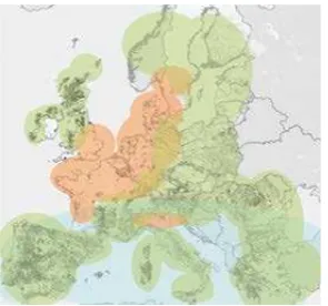
Figure 1. Environmental challenges for European agriculture (EEA, 2012)
On Figure 1. the most substantial agricultural areas are shown with green colour, displaying the main challenges as follows: it is important to maintain on-field biodiversity, stimulate
* Corresponding author
favourable practices, increase profitability without intensifying agricultural activities. (EEA, 2012)
In our paper we would like to propose a dynamic method with agent-based modelling to find the most problematic areas where these actions are essential.
2. MODELLING ENVIRONMENT
The outlined ‘greening’ policy and its solution can be successfully achieved by complex use of GIS methods and modelling tools. As opposed to the usual statistical analysis of a chosen area (a standard GIS procedure) our aim is to model the current situation and to obtain an accurate numeric potential map (landscape heterogeneity map) that can objectively show the diversity of a test area. We combined the GIS data with a high-level programming language called NetLogo, and estimated the results by simulation called agent-based modelling (ABM).
2.1 Agent-based modelling
An agent is an entity that can perceive its environment through sensors and can act upon that environment through actuators. A human agent has eyes, ears, and other organs for sensors and hands, legs, mouth, and other body parts for actuators. (Russel and Norvig, 2003)
The concept of rationality can be applied to a wide variety of agents operating in an imaginable environment. (Russel and Norvig, 2003). The term agent-based modelling (ABM) refers to the use of computational methods that are created to investigate processes and problems viewed as dynamic systems of interacting agents. An example might be attempting to model crowd behaviour in a football stadium using computational agents to represent individuals in the crowd. (de Smith, M.J. et al., 2015).
2.2 Software components
As a primary tool to handle the input raster data, QGIS (free and open source Geographic Information System) was used in addition to its Python API (Application Programmer Interface) called PyQGIS. (Sherman, 2014). GDAL (Geospatial Data Abstraction Library) library functions were called in batch processing to clip out the raster worlds. The exported raster files were then imported into NetLogo, which is a multi-agent programmable modelling environment. (Wilensky, 1999). Moreover, we have extended the functionality of NetLogo (further NL) with Wolfram Mathematica. These tools provide easy to use, real-time analysing capability which is far superior to individual applications supplementing the abovementioned program. (Bakshy and Wilesky, 2007). The final products are derived from the analytical procedure - such as diversity contour maps - were obtained in QGIS. The following figure shows the sequence and architecture of the data processing programs.
Figure 3. An overview map of the software components
2.3 Input data
The CORINE Land Cover (CLC) is referring to a European programme establishing a computerised inventory on land cover of the 27 EC member states and other European countries. (Wiki CORINE, 2015) This data are available in 100 meters resolution and it is being categorized into 44 classes of the 3-level CORINE nomenclature. The CLC raster data was last uploaded in 2009 in a Lambert Azimuthal Equal Area projection.
2.4 Test area
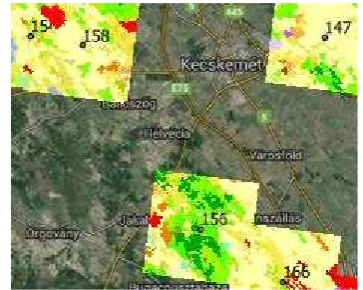
A part of the Great Hungarian Plain was selected as a test area. The CORINE raster dataset was subdivided into smaller parts to form NetLogo worlds – for example No. 156 in Figure 3. A world is the basic unit of the simulation where the agents act. The centre points of the worlds were randomly distributed in the test area and afterwards the clipper window defined their extension.
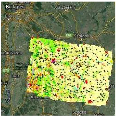
Figure 4. Some extracted worlds (from CORINE) with identifiers, GoogleMaps layer in background, scale 1:800 000,
near the city of Kecskemét
3. METHODOLOGY
3.1 Landscape scout agent
We defined the properties of an agent whose aim is to map the total diversity of a particular land (world). The agent keeps moving all the time, hence it moves on to continuously discover the true landscape.
Moreover, the agent has the following properties:
• Has a memory: i.e. a specified type of land cover (e.g. pasture) is only registered once.
• Can see in a conic shape field of view.
• Has a knowledge base about the states which leads to actions with a probabilistic nature.
• It always chooses the shortest way to reach a new type of land cover.
• Registers and collects the unique land covers into a common sum as a Monte Carlo integral.
Figure 5. The agent sees in a cone - illustration (defined by opening angle and distance parameters)
By simulating the agents’ movement, the following formula can describe the position of an agent at a particular time:
�(�,�) = {�,�}
�: ℤ2→ ℝ2 (1)
where the i is the identifier of the agent, the t is the epoch of simulation. There can be a finite land cover type in the investigated worlds:
The CLC raster model orders land cover classes to the coordinates of the worlds introduced in Figure 4:
�(�, {�,�}) =�
�: ℝ3→ � (3)
The cluster function’s (3) arguments are the � (theta) as world identifier, and the agent’s coordinates {x, y}. During the simulation an agent walks along a path and records the land cover observations into a sequence:
(���,�)�=0� , ���,�=���,�(�,�)� (4)
where d means the length of simulation in time periods (ticks). As it was mentioned, an agent has a memory (stores the visited cells' data) so its motion is path dependent:
�(�,�,�) =�� ∈ �� (���,�)�=0� � (5)
Considering the status of the newly visited states, there are two possibilities:
1. The agent detects a new type of land cover. The possible actions in the state:
a. The agent faces to the closest point of the new land cover with 95 % probability and will move to the adjacent cell in forward direction. (Briefly in NL: face min-one-of patches in-cone 50 120 with [not member? covername mem] [distance myself]].) b. It will rotate randomly with 5 % probability
(according to normal distribution) and will make one step in the rotated direction. 2. There is not any new type of land cover in the conic
horizon (considering 50 cells in forward direction and 120• of opening angle of a conical shaped viewing space). There can be two actions performed by the agent:
a. Rotate randomly with 80 % probability and move.
b. Will not rotate but will move forward with 20% probability
The abovementioned algorithm implies that the agent's primary goal is to detect the unvisited land as quickly as possible (forward progression has much larger probability than rotation), assuming that the land stretches over multiple pixels. Rotation provides the possibility of discovering adjacent cells or exploring areas in different direction. In case of forward movement, the agent will make a step of one pixel. These partly stochastic mechanisms determines the path of a particular scout. Whilst the agents route their paths the newly appeared land covers are counted:
�(�,�,�) =�1 ,�����,�(�,�)� ∉ �(�,�,� −1) 0 ,�����,�(�,�)� ∈ �(�,�,� −1)
�: ℤ3→{0,1}
(6)
The landscape diversity is capable to describe with a potential value that is calculated by summing up the newly appeared land covers per agents as a Monte Carlo integral:
�(�,�,�) =� � �(�,�,�)
where a is the number of scout agents and d is the duration of simulation. The equation expressed the diversity potential of a particular world. By selecting some worlds in a workspace the modeller can calculate their potential, and create a potential map from the sample points. The map will cover the investigated area. In the following sections the simulation results will be described.
4. DISCUSSION - SIMULATION
4.1 Test world
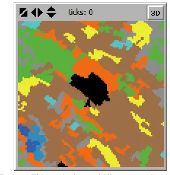
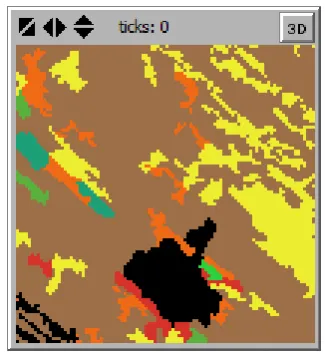
The following figure shows a test world without agents. The colour schema is obtained from the colour table of the NetLogo model.
Figure 6. This particular world lies next to the city of Kecskemét and a town called Kerekegyháza can be seen in the
middle
The ticks in the middle show the current epoch of simulation. Converting the CORINE grid codes to land cover names according to the 2-level CORINE nomenclature labels the following distribution of land covers can be observed:
Table 1. The introduced world seem to very heterogeneous, it consists nine land cover types
4.2 Introduction of scouts' motion
The landscape scouts' aim is to collect as many land cover types it is possible. The following figure shows how the agents keep discovering a new type of land making a unique path which is highly dependent on the original position and orientation.
Figure 7. The path of agent that always moves toward an unvisited type of land. Having visited all possible land types, it
starts wandering.
The origin of discovery started from the forest, then the agent moved into the orange area (the arable land), followed by pasture (yellow) and so forth. This path can be read out from the memory of the agent as follows:
["forests", "heterogeneous agricultural areas", "arable land" "pastures", "permanent crops", "scrub and or herbaceous vegetation associations", "urban fabric", "inland wetlands", "inland waters"]
After the discovering period – the first 100 ticks -, we can see a wandering period - which implies the lack of new neighbouring land cover clusters. We can conclude that our "discoverer" agent has collected each type of cover resulting 8 in the integral – since the origin does not count. According to the diversity report: [[100 7] [200 8]] – read that after 100 periods (number of ticks) the agent collected the most type.
5. DISCUSSION
5.1 Novelty of method
The standard statistical analysis cannot always describe the land
has to consider the number of occurring land covers (cardinality), their distribution, borders or perimeters. Moreover, even their neighbouring properties could count, so the spatial autocorrelation must also be taken into consideration (Moran's I).
Figure 8. The white and black squares are perfectly dispersed.
On Figure 8. we illustrated a very odd distribution of two alternating land cover types (chessboard), with maximal heterogeneity and border sum. It would yield to a maximum potential if our agents did not have a memory, i.e. they could revisit the same land cover type many times. This would be clearly useless, because this regular chessboard type landscape cannot be viewed as a very diverse one. This regular pattern could be merged into each other on the ground.
Considering all these, we have chosen a dynamic method which is the agent-based modelling.
5.2 Parameters of agent-based modelling
In agent-based modelling we must consider the number of agents and simulation length in time (ticks).
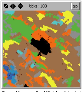
Figure 9. Shows 50 scouts after 100 ticks of simulation on the sample world
The running time of the algorithms with 100 agents for 50 ticks or 50 agents for 100 ticks are roughly identical. After the simulation we can read out the potential of the test area introduced in Eq. 7.
5.3 Simulation on workspace
Figure 10. The random distribution of world centres over the area.
Then we calculated each world’s landscape diversity with the outlined method.
Figure 11. The histogram about the workspace diversity, created from 400 length sample (worlds are shown in Figure 10.)
To compare the simulation results and to prove its robustness we would like to introduce the concept of a highly diverse world as opposed to a low diversity world.
5.4 Comparison of worlds
In this section we would like to test whether the accuracy of ABM algorithm depends on the diversity of the world. In order to check this, we collected 3 types of worlds (from the worlds of Figure 10.).
First we introduce the lowest diversity workspace as it is shown in Figure 12. It has a cardinality of 3 and a potential value of 92.
Figure 12. Least diverse world of workspace.
We create a sample of 10 elements by rerunning the simulation on the world shown on Figure 12.
Figure 13. Histogram of a low diversity world of workspace.
The relative mean deviation of the algorithm in case of a low diversity world was calculated by dividing the mean deviation with the arithmetic mean (where n represents the sample length, the x is the potential):
���=
1
� ∑��=1|��− �̅|
�̅ =
1.44
90.7= 0.0159
(8)
As one can observe, the relative mean deviation for the simulation is rather small.
Figure 14. An average diverse world of workspace.
Instead of the available maximum potential which is 350 in this case (one agent can collect 7 additional land cover types, in addition to its original land cover type that has been listed), there are 7 new more land cover types that can be discovered. All together 50 agents on 8 different land cover types can collect 50*7 potentials which is equal to 350, the agents reach only approximately 274.
���= 3.82
274.435�����������= 0.0139
The relative mean deviation is still low, even though the agents can accumulate much higher potential value.
In the next step we continue the comparison with the most diverse world with the potential of 400, where the possible maximum potential is 450 units (land cover cardinality is 10).
Figure 15. The landscape heterogeneity - recorder world with the highest potential.
Table 2. Land cover occurrences
The third type of land yielded a low relative mean deviation as well:
���= 6
391.6
�������= 0.0153
The algorithm which has some stochastics part converges to a particular value, implying deterministic nature of the process. We can say that the relative error of the method is rather small, only 1 % on each land cover type.
5.5 Land cover cardinality
One could easily assume that the diversity potential only depends on the number of land cover types existing in a given world. However, it is not really the case, nevertheless there is a correlation between the cardinality (number of land cover types) and the potential.
The following figure demonstrates this situation.
Figure 16. The relationship between landscape potential and cardinality
It can be seen from the figure that a given potential value (i.e. 250) can be observed in different worlds (cardinalities 6, 7, 8, 9 and 10), so it is not a one-to-one relationship. Surprisingly the highest potential world comes from the 10 cardinality bucket, not from the world with maximal cardinality (11 in our case). Finally we calculated a Pearson's correlation coefficient to express the strength of the correlation:
�=���= ∑ (��− �̅)(��− ��)
� �=1
�∑��=1(��− �̅)2�∑��=1(��− ��)2= 0.791 (9)
where n represents the sample size, x is the potential value and y is the cardinality of the dataset.
Analysing Figure 16. we can find a world with cardinality of 5 whose potential is similar to a world with cardinality of 9. This fact could be explained by an uneven distribution of the unique land covers.
6. MAPPING THE RESULT
After the collection of diversity potential points a potential contour map was created by the Interpolation and Contour QGIS Plugin. The plugin first generates a triangulated irregular network (TIN) by Delaunay triangulation which yields to a surface formed by triangles of nearest neighbour points. Having obtained the triangulated irregular network, potential contour lines were calculated on the workspace. The used contour interval equals to 25 potential units.
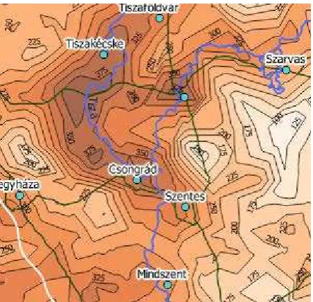
Figure 17. The Danube–Tisza Interfluve on scale 1:750 000. The thematic layers: blue lines – rivers; white – motorway, green – primary road; towns and cities with white shadow.
The darker red colour means that the given area possesses a higher potential value, which implies more heterogeneity. On the other hand, lighter colours will correspond to the low landscape diversity, which means that the area is problematic. The interventions by authorities or farmers are necessary on the lower potential fields (areas with light colours). The Tiszántúl or Transtisza, the area which lies east from the river Tisza shows lower values (problematic region) which truly coincides with the real situation.
7. SUMMARY
By dynamic agent-based modelling a map of the landscape diversity potential was obtained, which looks similar to the regular topographical maps. However, in this case colour intensity refers to landscape heterogeneity rather than to elevation.
This map can be used by decision makers to support farming according to measurable and objective criteria, where the goal is to increase landscape heterogeneity and diversity. Because of the algorithm proved to be robust, it can be used with high reliability.
Figure 18. The Danube–Tisza Interfluve and Transtisza
REFERENCES
Bakshy, E., Wilensky, U., 2007. NetLogo-Mathematica Link. http://ccl.northwestern.edu/netlogo/mathematica.html. Center for Connected Learning and Computer-Based Modeling, Northwestern University, Evanston, IL.
Corine Land Cover - OpenStreetMap Wiki, 2015. http://wiki.openstreetmap.org /wiki/Corine_Land_Cover
de Smith, M.J., Goodchild, M.F., Longley, P.A., 2015. Geospatial Analysis, Fifth Edition, The Winchelsea Press, Winchelsea, UK
European Environment Agency (EEA), 2014. Greening Europe’s agriculture, http://www.eea.europa.eu/themes/agriculture/ greening-agricultural-policy
European Environment Agency (EEA), 2012. Agriculture and the green economy, http://www.eea.europa.eu/themes/ agriculture/greening-agricultural-policy/greening-the-cap-paper
Sherman, G., 2014. The PyQGIS Programmer's Guide
Russel, S., Norvig, P., 2003. Artificial Intelligence: A Modern Approach, Prentice Hall, New Jersey
Wilensky, U., 1999. NetLogo, Center for Connected Learning and Computer-Based Modeling, Northwestern University, Evanston, IL. http://ccl.northwestern.edu/netlogo/.