LINE-BASED REGISTRATION OF DSM AND HYPERSPECTRAL IMAGES
J. Avbelja,b, D. Iwaszczukc, R. M¨ullera, P. Reinartza, U. Stillac aGerman Aerospace Center, Oberpfaffenhofen, 82234 Weßling
-(janja.avbelj, rupert.mueller, reinartz)@dlr.de b
Chair of Remote Sensing Technology, Technische Universit¨at M¨unchen, Arcisstr. 21, 80333 M¨unchen cPhotogrammetry and Remote Sensing, Technische Universit¨at M¨unchen, Arcisstr. 21, 80333 M¨unchen
-(dorota.iwaszczuk, stilla)@tum.de
KEY WORDS:Hyper spectral, DEM/DTM, Registration, Multisensor, Urban, Matching, LiDAR
ABSTRACT:
Data fusion techniques require a good registration of all the used datasets. In remote sensing, images are usually geo-referenced using the GPS and IMU data. However, if more precise registration is required, image processing techniques can be employed. We propose a method for multi-modal image coregistration between hyperspectral images (HSI) and digital surface models (DSM). The method is divided in three parts: object and line detection of the same object in HSI and DSM, line matching and determination of transformation parameters. Homogeneous coordinates are used to implement matching and adjustment of transformation parameters. The common object in HSI and DSM are building boundaries. They have apparent change in height and material, that can be detected in DSM and HSI, respectively. Thus, before the matching and transformation parameter computation, building outlines are detected and adjusted in HSI and DSM. We test the method on a HSI and two DSM, using extracted building outbounds and for comparison also extracted lines with a line detector. The results show that estimated building boundaries provide more line assignments, than using line detector.
1 INTRODUCTION
Data fusion is widely used in variety of fields and applications in science and engineering. It is an important procedure for in-tegration and analysis of many datasets in photogrammetry, re-mote sensing and computer vision. Data fusion of rere-mote sens-ing data becomes notably challengsens-ing while integratsens-ing data from different sensors, mounted on different platforms and collected in different points in time. Typically the acquired data is geo-referenced, but often the accuracy of the geo-referencing is not sufficient to achieve the best possible fit between all data sets. The geometric inaccuracies of data integration can lead to diffi-cult or even impossible interpretation of fused result. Therefore, coregistration of all datasets has to be carried out before the fu-sion. For multi-modal image registration, methods using mutual information are widely used in remote sensing as well as in med-ical imaging (Pluim et al., 2003).
The aim of our work is multi-modal coregistration of hyperspec-tral images (HSI) with digital surface model (DSM) in image space using line features. Focusing on urban areas, a high vari-ety of objects is present in a scene having different sizes, shapes, heights and materials. Common features or characteristics of both datasets must be found to estimate the transformation parameters. On one hand, HSI are optical images describing spectral charac-teristics of each pixel with high spectral resolution. Every ma-terial is uniquely described with a spectral signature and can be compared to the spectra in HSI. Thereby material of each image pixel can be defined. On the other hand, DSM show heights of the observed areas and objects in them. The objects, such as streets, buildings and bridges can be detected in HSI, because they are often built from a material different from surroundings. In DSM object detection is possible as well as predication about objects height and geometry. Fusion of these both datasets contributes to better interpretation and is expected to increase the detection rate.
Buildings and other man-made objects are mainly linear struc-tures. Therefore, for description and coregistration of data cap-tured in urban areas many authors propose lines or line segments (Stilla, 1995, Schenk, 2004, Debevec et al., 1996, Iwaszczuk et
al., 2012, Ok et al., 2012). However, each detected line has a different accuracy depending on used data and detection method. This accuracy should also be taken into consideration for istration. Accordingly we present a method for line-based coreg-istration of DSM and HSI data with respect to the accuracy of the linear features. We define the affine transformation between the data sets. As described in (Hartley and Zisserman, 2004) and (Zeng et al., 2008) affine transformation can be calculated from line correspondences using direct linear transformation method (DLT), but they do not introduce the accuracy of the used lines. What is more, we propose detecting lines as building outbounds in HSI and DSM, and so incorporating also topology knowledge (Avbelj, 2012).
2 OBJECT AND LINE DETECTION
2.1 Material Selection and Material Map Generation
Some of the pixels in HSI consist of more than just one material, called mixed pixels. If a complete collection of materials with spectral signatures is known, then the fractions of materials can be computed for every HSI pixel. Common procedure to decom-pose each measured pixel into the constituent spectra is spectral unmixing (Keshava, 2003). If spectra of few target materials are known the unmixing does not provide reliable result. Neverthe-less, the similarity between known spectra and image spectra can be computed. Such similarity measures are for example euclidean distance or distances designed especially for HSI data, the Spec-tral Angle Mapper (SAM) (Kruse et al., 1993) and SpecSpec-tral In-formation Divergence (Chang, 2000). We choose SAM similarity measure because it is nearly insensitive to illumination, however any other similarity measure or spectral unmixing result could be used. SAM is computed as
SAM(r,t) = cos−1
same and completely dissimilar spectra, respectively.
The spectral signatures of roofing materials present in the scene, which seldom appear on the ground, such as copper and ceram-ics tiles, are manually collected in HSI. Then the SAM between known material spectra and each pixel is HSI is computed. So, for every chosen roofing material the material map with similarity distances is computed.
2.2 Line Detection
Line segments are needed, to establish correspondence between a HSI and height image. The lines are detected in height data and in material maps, but not directly in HSI. The material map calculated as proposed in 2.1 are material maps of roofing ma-terials, therefore lines on building boundaries are of our interest. So, we detect the building outlines and use them for line assign-ment. For a comparison, we extract the line segments also with a linear-time line segment detector (von Gioi et al., 2010). Line as-signment and transformation parameters are calculated for both, extracted outbounds and extracted lines.
2.2.1 Building Outline Detection consists of three steps: a) building mask extraction, b) building model selection, and c) boundary adjustment. Many building detection and modelling methods were proposed in last decades, e.g. (Maas and Vossel-man, 1999) proposed a method for building modelling from high resolution LiDAR data, whereas (Sohn and Dowman, 2007) used multispectral and height data for extraction of buildings. In this section, we only summarize the building outline detection, be-cause it exceeds the scope of this paper.
a) An initial guess for building regions is a building mask. From DSM, a building mask is extracted by normalizing the DSM, defining the above-ground objects and removing the high vege-tation. In HSI, the building mask is defined by automatic thresh-olding material map. The threshold is set to 3σfrom selected material pixels.
b) We assume buildings can be composed from rectilinear shapes. Under this assumption, every building can be reconstructed by subtracting and adding rectangles. Such hierarchical approach for building outline detection is proposed by (Gerke et al., 2001), but we use model selection instead of fixed threshold of mini-mum area to be estimated. For every building region in the build-ing mask, a set of models is build. First, the model of level one
ml = 1is build as a minimum bounding box of a region. Then, the rasterized minimum bounding box is subtracted from the building mask. If there are any remaining pixels, the bound-ing boxes of them are computed, and buildbound-ing model of level two = 2 is computed. Furthermore, the models are iteratively build until no regions are left to approximate. Before the model of higher level is build, the boundaries are adjusted as described in c). Final, the optimal model is selected as a trade off between complexity and best fitting model. The Model Complexity is computed as
M odelComplexity=√mlRM S(ri,ml) (2)
whereri,mis the shortest distance between the border pixeliof the building mask and building model lines of levelml,mlis the model level, and RMS is a root mean square value of distance vectorri,ml.
c) Every line segment of the selected building model is adjusted according to the image gradients using gradient descend method.
The new line segments are intersected to produce the building outline. Lines shorter than 3 pixels are not adjusted, and building polygon is regularized by joining subsequent lines with intersec-tion angle smaller than 10◦.
2.2.2 The linear-time line segment detector (LSD) partitions the image into line-support regions according to the proximity and gradient angle, then finds the line segments best approximat-ing each of these regions and lastly, validates each line segment according to the line-support region (von Gioi et al., 2010).
3 MATCHING OF HSI AND HEIGHT DATA
3.1 Line assignment
Both algorithms, line detection and building outline detection, re-sult in sets of lines in both data sets, HSI and hight data. Accord-ing to the imperfect geo-referencAccord-ing of the data and inaccurate line detection, a tipical mismatch between the line segments ex-ists. The range of this mismatch depends mostly on the accuracy of geo-referencing. We propose a method which can be applied also for data where the relative error of geo-referencing between the data sets amounts to 20-30 image pixels or even larger.
We implemented an automatic approach using a 3D accumulator for line matching. We use one of the data sets as reference and move line segments from the second data set over the line seg-ments from the first data set. For each position we check how many lines correspond to each other and fill accumulator with this number. At the same time we store the line correspondences for this position. We repeat this procedure rotating line segments from the second data set by small angles in range of few degrees. This algorithm results in an 3D accumulator filled with number of fitting lines for each line correspondences assigned to each cell of accumulator. Then we search for the cell with maximal number of correspondences in accumulator and use line correspondences assigned to this cell for transformation parameter calculation.
The correspondence between the lines for every position and an-gle of the accumulator is determined using statistical tests. We use homogeneous coordinates to implement the problem. As shown in (Heuel, 2002) we calculate the distance vectord and test the hypothesisH0
H0:d= U(x)y= V(y)x=0 (3)
wherexandyare entities and U and V are functions defining the relation betweenxandy. In this particular casexandyare lines and we investigate their incidence. Further on, we calculate the covariance matrix for the distance vectord
Σdd= U(x)ΣyyUT(y) + V(x)ΣxxVT(y). (4)
Then we rejectH0with the significance levelαif dTΣ−1
ddd> ǫH=χ21−α;n. (5)
3.2 Determination of transformation parameters
Selected correspondences are used for determination of the trans-formation matrixH. We set our functional model as
m= H−T l⇒HT
m=l (6)
wheremrepresents a line segments from the reference data set and lrepresents a line segments from the second data set (see (Hartley and Zisserman, 2004), p.36, Eq. 2.6 ). We assume that mandlrepresent the same line, so the condition for the identity relation is
HT
m×l= 0. (7)
Then we define transformationHas affine transformation
H =
We calculate lines as joint of two end points of detected line seg-mentse1ande2
l=e1×e2 (9)
and normalize spherically
N(l) = l
|l|. (10)
Finally we estimate optimal affine transformation using Gauss-Helmert model. We set conditions
g(ˆb,ˆp) = HTm×l= 0 (11)
Three datasets of a residential area of the city of Munich are used to demonstrate the proposed coregistration method. First dataset, HSI was acquired with a HySpex hyperspectral camera. The system consists of two sensors, VNIR and SWIR camera, providing two images that are combined in a postpocessing step. For the tests we used the VNIR image only with 160 channels in a spectral range of 410-990 nm, and 3.7 nm sampling inter-val. Four channels were removed before processing due to the high noise level. Second dataset, 3K DSM was computed from multi-view optical images using semi global matching. The op-tical images were acquired with the 3K camera system, consist-ing of three non-metric cameras, one nadir lookconsist-ing and, and two looking oblique sidewards. The 3K system has a GPS/INS unit and was developed at DLR IMF (Kurz et al., 2012). HSI and 3K images have a spatial resolution of 2 m. Third dataset is a LiDAR DSM with 1 m spatial resolution. It is resampled from the Li-DAR point cloud with an average density of 1.69 pixels/m2with the nearest neighbour method.
4.2 Experimental Results
Material maps of three most common roofing materials present in the HSI, i.e. red roof tiles, concrete and copper, are com-puted from manual selected spectra. For each material, ten tra are collected and averaged to obtain reference material spec-tra (Fig. 1). Averaging selected image specspec-tra over few pixels
suppresses possible noise, and is more reliable then using just a single HSI pixel. Spectral signatures in Fig. 1 have some sharp edges, indicating systematic noise in the HSI. This spectral inac-curacies do not significantly influence the material map computa-tion, because SAM is computed between collected image spectra from HSI and the pixels of the same HSI. On the contrary, using existing spectral library spectra and HSI with some systematic errors, e.g. not sufficiently corrected atmospheric or radiometric influence, would influence the material map computation.
Figure 1: Spectral signatures of three roofing materials.
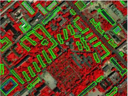
Figure 2: Detected buildings (green) in HSI. False colour com-posite image with channels of wavelengthλ= 0.66, 0.51 and 0.45
µm.
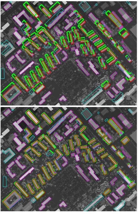
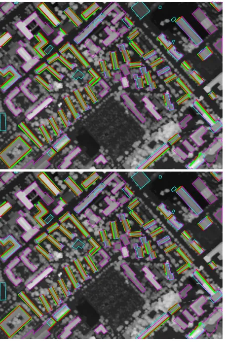
Building outlines and lines are extracted in HSI (Fig. 2), LiDAR DSM (Fig. 3, 4) and 3K DSM (Fig. 5, 6). Then, line assignment and coregistration is computed twice for both pairs of images, i.e. LiDAR DSM - HSI and 3K DSM - HSI; First with extracted building outbounds and second with detected lines with LSD. For line matching the building outbounds are considered to be line segments without topology.
Proposed building outbound detection delivers large enough num-ber of approximate buildings for line assignment and coregis-tration. In addition, more assignments are found between the extracted building outbounds than between extracted lines with LSD (Fig. 3-6). Majority of the adjusted buildings are approx-imated with an appropriate model. However, in all three used datasets, some buildings partly present in the image are badly es-timated or not eses-timated at all. In Fig. 2 the number of extracted building outbounds is not complete, because only three roof ma-terials were considered. To increase the completeness of building extraction, all building materials in the given scene should be col-lected.
Figure 3: Detected buildings in LiDAR DSM and HSI, before (top) and after coregistration (bottom). Red: lines detected in LiDAR data matched with lines detected in HSI. Cyan: lines de-tected in HSI without any matches found in DSM. Magenta: lines detected in LiDAR DSM without any matches found in HSI .
(Eq. 8) for LiDAR DSM and HSI, and for 3K DSM and HSI are listed in Tab. 1 and 3. The parametersh3 and h6 are the translations inxandydirection in pixels of a reference image; This is 1 m for LiDAR DSM and 2 m for 3K DSM. The other four
haffine parameters are without units. The initial registration of LiDAR DSM and HSI was corrupted to demonstrate effectiveness of the accumulator. The initial registration of 3K DSM and HSI was already on a pixel level. In all tests, the significance levelα
= 0.08 (Eq. 5) is set for testing the correspondence between lines.
Buildings Lines
h1±σh1 0.9971±0.0004 0.9986±0.0005
h2±σh2 -0.0008±0.0006 -0.0015±0.0007
h3±σh3 12.4056±0.0732 12.1408±0.0882
h4±σh4 0.0010±0.0004 0.0017±0.0004
h5±σh5 0.9994±0.0006 0.9987±0.0007
h6±σh6 12.7813±0.0758 12.2797±0.0939 Table 1: Estimated affine parameters for LiDAR DSM and HSI using extracted building outlines and lines.
Estimated affine parameters for LiDAR DSM - HSI coregistra-tion, using building outbounds or lines are comparable, the stan-dard deviations of allhparameters are slightly smaller (Tab. 1). Same holds true for the 3K DSM - HSI coregistration (Tab. 3).
To evaluate the estimate affine parameters, 83 points were man-ually measured in HSI and LiDAR DSM (Tab. 2). Parameters
Figure 4: Detected lines in LiDAR DSM and HSI, before (top) and after coregistration (bottom). Line colours as described in Fig. 3.
Manual Points
h1±σh1 0.9957±0.0006
h2±σh2 -0.0023±0.0008
h3±σh3 14.8674±0.2874
h4±σh4 0.0030±0.0008
h5±σh5 1.0026±0.0006
h6±σh6 11.3304±0.2874
Table 2: Estimated affine parameters for LiDAR DSM and HSI with manual selected tie points.
Buildings Lines
h1±σh1 1.0010±0.0006 1.0015±0.0008
h2±σh2 -0.0017±0.0010 0.0002±0.0012
h3±σh3 0.1629±0.0639 1.7865±0.0711
h4±σh4 0.0027±0.0007 0.0018±0.0008
h5±σh5 1.0005±0.0010 0.9999±0.0014
h6±σh6 -0.8919±0.0698 0.2276±0.0772 Table 3: Estimated affine parameters for 3K DSM and HSI using extracted building outlines and lines.
Figure 5: Detected buildings in 3K DSM and HSI, before (top) and after coregistration (bottom). Line colours are analogue to description under Fig. 3.
coregistration method.
5 DISCUSSION AND FUTURE WORK
We proposed a method for coregistration of HSI and DSM us-ing lines from detected buildus-ing outbounds usus-ing homogeneous coordinates for line assignment and transformation parameter es-timation. The method can be applied on multi-modal and multi resolution datasets. Estimating building outlines instead of lines provide larger amount of assigned lines between the images, and is thus more reliable to estimate transformation parameters.
Detecting only the lines belonging to the same object in HSI and DSM allows incorporating prior knowledge about the observed object. For example, rectilinearly of building boundaries can be introduced to improve the building outline detection and conse-quently transformation parameter estimation. Additional knowl-edge about shapes of observed object is specially important for images with lower spatial resolution or for automatic generated DEM with missing values.
For more efficient line assignment, building outlines with topol-ogy should be implemented. Furthermore, the building outline detection with model selection must be evaluated for positional accuracy of detected lines. Introducing these line accuracies into the determination of transformation parameters showed good re-sults, so investigations about influence of line accuracies on trans-formation parameters will be carried out.
Figure 6: Detected lines in 3K DSM and HSI, before (top) and after coregistration (bottom). Line colours are analogue to de-scription under Fig. 3.
REFERENCES
Avbelj, J., 2012. Spectral information retrieval for sub-pixel building edge detection. ISPRS Annals of Photogrammetry, Re-mote Sensing and Spatial Information Sciences I-7, pp. 61–66.
Chang, C.-I., 2000. An information-theoretic approach to spectral variability, similarity, and discrimination for hyperspectral im-age analysis. IEEE Transactions on Information Theory 46(5), pp. 1927–1932.
Debevec, P., Taylor, C. and Malik, J., 1996. Modelling and ren-dering architecture from photographs: a hybrid geometry- and image-based approach. In: Proceedings of the 23rd Annual Conference on Computer Graphics and Interactive Techniques, pp. 11–20.
Gerke, M., Straub, B. M. and Koch, A., 2001. Automatic de-tection of buildings and trees from aerial imagery using different levels of abstraction. Publications of the German Society for Pho-togrammetry and Remote Sensing 10, pp. 273280.
Hartley, R. I. and Zisserman, A., 2004. Multiple View Geometry in Computer Vision. Second edn, Cambridge University Press, ISBN: 0521540518.
Iwaszczuk, D., Hoegner, L., Schmitt, M. and Stilla, U., 2012. Line based matching of uncertain 3d building models with ir im-age sequences for precise texture extraction. Photogrammetrie, Fernerkundung, Geoinformation (PFG) 2012(5), pp. 511–521.
Keshava, N., 2003. A survey of spectral unmixing algorithms. Lincoln Laboratory Journal 14(1), pp. 5578.
Kruse, F., Lefkoff, A., Boardman, J., Heidebrecht, K., Shapiro, A., Barloon, P. and Goetz, A., 1993. The spectral image process-ing system (SIPS)interactive visualization and analysis of imag-ing spectrometer data. Remote Sensimag-ing of Environment 44(2-3), pp. 145–163.
Kurz, F., T¨urmer, S., Meynberg, O., Rosenbaum, D., Runge, H., Reinartz, P. and Leitloff, J., 2012. Low-cost optical camera sys-tems for real-time mapping applications. PFG Photogrammetrie, Fernerkundung, Geoinformation 2012(2), pp. 159–176.
Maas, H.-G. and Vosselman, G., 1999. Two algorithms for ex-tracting building models from raw laser altimetry data. ISPRS Journal of Photogrammetry and Remote Sensing 54(23), pp. 153– 163.
Ok, A., Wegner, J., Heipke, C., Rottensteiner, F., S¨orgel, U. and Toprakc, V., 2012. Matching of straight line segments from aerial stereo images of urban areas. ISPRS Journal of Photogrammetry and Remote Sensing 74, pp. 133–152.
Pluim, J. P. W., Maintz, J. B. A. and Viergever, M. A., 2003. Mutual-information-based registration of medical images: a sur-vey. Medical Imaging, IEEE Transactions on 22(8), pp. 9861004.
Schenk, T., 2004. From point-based to feature-based aerial trian-gulation. ISPRS Journal of Photogrammetry and Remote Sensing 58, pp. 315–329.
Sohn, G. and Dowman, I., 2007. Data fusion of high-resolution satellite imagery and LiDAR data for automatic building extrac-tion. ISPRS Journal of Photogrammetry and Remote Sensing 62(1), pp. 43–63.
Stilla, U., 1995. Map-aided structural analysis of aerial images. ISPRS Journal of photogrammetry and remote sensing 50(4), pp. 3–10.
von Gioi, R., Jakubowicz, J., Morel, J.-M. and Randall, G., 2010. LSD: a fast line segment detector with a false detection control. IEEE Transactions on Pattern Analysis and Machine Intelligence 32(4), pp. 722 –732.