Contents lists available atScienceDirect
Applied Mathematics Letters
journal homepage:www.elsevier.com/locate/aml
Weak local residuals as smoothness indicators for the
shallow water equations
Sudi Mungkasi
a,∗, Zhenquan Li
b, Stephen Gwyn Roberts
caDepartment of Mathematics, Sanata Dharma University, Mrican, Tromol Pos 29, Yogyakarta 55002, Indonesia
bSchool of Computing and Mathematics, Charles Sturt University, Thurgoona, NSW 2640, Australia
cMathematical Sciences Institute, The Australian National University, Canberra, ACT 0200, Australia
a r t i c l e i n f o
Article history:
Received 26 October 2013
Received in revised form 12 December 2013 Accepted 12 December 2013
Keywords:
Weak local residual Smoothness indicator Shock detector Finite volume method Shallow water equations Conservation laws
a b s t r a c t
The system of shallow water equations admits infinitely many conservation laws. This pa-per investigates weak local residuals as smoothness indicators of numerical solutions to the shallow water equations. To get a weak formulation, a test function and integration are introduced into the shallow water equations. We use a finite volume method to solve the shallow water equations numerically. Based on our numerical simulations, the weak local residual of a simple conservation law with a simple test function is identified to be the best as a smoothness indicator.
©2013 Elsevier Ltd. All rights reserved.
1. Introduction
Weak local residuals as smoothness indicators or shock detectors for conservation laws were proposed by Karni, Kurganov and Petrova [1,2]. They proved that weak local residuals have higher accuracy on smooth regions than nons-mooth regions. This difference in accuracy makes weak local residuals able to detect the snons-moothness of numerical solutions and the presence of shock waves. Therefore, weak local residuals are good candidates as refinement indicators for adaptive numerical methods used to solve conservation laws.
In this paper we limit our discussion on the shallow water equations without source terms. We investigate weak local residuals of conservation laws relating to the shallow water equations. Note that these equations admit infinitely many conservation laws as described by Whitham [3]. In formulating the weak local residual, we introduce a test function and integration. Our goal is to find which conservation law of the shallow water equations and which test function should be chosen in order to get a reliable smoothness indicator with the cheapest computation possible.
The rest of this paper is organized as follows. Section2presents formulations of weak local residuals of conservation laws. Conservation laws admitted by the shallow water equations are provided in Section3. Following that, Section4reports our numerical experiment results on weak local residuals as smoothness indicators of the shallow water equations. Finally, some concluding remarks are drawn in Section5.
2. Weak local residuals
Consider the scalar conservation law with an initial condition
qt
+
f(
q)
x=
0,
−∞
<
x<
∞
,
q
(
x,
t)
=
q0(x),
t=
0.
(1)∗Corresponding author. Tel.: +62 81328006324.
E-mail addresses:[email protected],[email protected](S. Mungkasi),[email protected](Z. Li),[email protected](S.G. Roberts). 0893-9659/$ – see front matter©2013 Elsevier Ltd. All rights reserved.
Herexis a one-dimensional space variable,tis the time variable,qis the conserved quantity,fis the flux function, andq0is
an arbitrary function defined for an initial condition. The weak form of the initial value problem(1)is
∞0
∞−∞
[
q(
x,
t)
Tt(
x,
t)
+
f(
q(
x,
t))
Tx(
x,
t)
]
dx dt+
∞−∞
q0(x
)
T(
x,
0)
dx=
0,
(2)whereT
(
x,
t)
is an arbitrary test function having compact support locally.Following Karni and Kurganov [2], we take uniform grids (xj
:=
j∆x,tn:=
n∆t) and letqnj be approximate values of
q
(
xj,
tn)
computed by a conservative method. We denote byq∆(
x,
t)
the corresponding piecewise constant approximation,q∆
(
x,
t)
:=
qnj if
(
x,
t)
∈ [
xj−1/2,xj+1/2] × [
tn−1/2,
tn+1/2]
(3)wherexj±1/2
:=
xj±
∆x/
2 andtn±1/2:=
tn±
∆t/
2. We construct a test functionTjn(
x,
t)
:=
Bj(
x)
Bn(
t)
, whereBj(
x)
andBn
(
t)
are quadraticB-splines centered atx=
xjandt
=
tnwith the support of size 3∆xand 3∆t. That is,Bj
(
x)
=
1 2
x
−
xj−3/2∆x
2ifxj−3/2
≤
x≤
xj−1/2,3 4
−
x−
xj∆x
2ifxj−1/2
≤
x≤
xj+1/2,1 2
x−
xj+3/2∆x
2ifxj+1/2
≤
x≤
xj+3/2,0 otherwise
,
(4)
andBn
(
t)
is defined similarly. Then substituting the test functionTnj
(
x,
t)
into(2)leads to a weak form of the local residualEjn
= −
tn+3/2tn−3/2
xj+3/2xj−3/2
q∆
(
x,
t)
Tjn(
x,
t)
t
+
f(
q∆
(
x,
t))
Tjn(
x,
t)
x
dx dt
,
(5)for conservation laws. After a straightforward computation, the weak local residual(5)can then be expressed as
Ejn
=
∆x12
qjn++11
−
qjn+−11+
4
qnj+1
−
qnj−1
+
qnj−+11−
qnj−−11
+
∆t12
f
(
qnj++11)
−
f(
qnj−+11)
+
4
f(
qnj+1)
−
f(
qnj−1)
+
f(
qjn+−11)
−
f(
qjn−−11)
.
(6)This taking of quadraticB-splines in constructing the test function adapts from the work of Karni, Kurganov and Petrova [1] on conservation laws. We denote by KKP (Karni–Kurganov–Petrova) indicator the weak local residual(6).
We can also choose the localized linearB-splines as the test functionsTjn+−11//22
(
x,
t)
:=
Bj+1/2(x)
Bn−1/2(
t)
, whereBj+1/2(x)
andBn−1/2
(
t)
are centered atx=
xj+1/2andt
=
tn−1/2with the support of size 2∆xand 2∆t. That is,Bj+1/2(x
)
=
x
−
xj−1/2∆x ifxj−1/2
≤
x≤
xj+1/2, xj+3/2−
x∆x ifxj+1/2
≤
x≤
xj+3/2,0 otherwise
,
(7)
andBn−1/2
(
t)
is defined similarly. This results in a less expensive computation of the weak local residualEjn+−11//22
= −
tn+1/2tn−3/2
xj+3/2xj−1/2
q∆
(
x,
t)
Tjn+−11//22
t
+
f(
q∆
(
x,
t))
Tn−1/2j+1/2
x dx dt
,
(8)which can be expressed after a straightforward computation as
Ejn+−11//22
=
∆x2
qnj
−
qnj−1+
qjn+1−
qnj+−11
+
∆t2
f
qnj+−11
−
f
qnj−1
+
f
qnj+1
−
f
qnj
.
(9)This taking of linearB-splines in constructing the test function adapts from the work of Constantin and Kurganov [4] on conservation laws. We denote by CK (Constantin–Kurganov) indicator the weak local residual(9).
We restate that in(2),T
(
x,
t)
is a locally supported test function. We see from the formulations of CK and KKP indicators, that CK indicator is simpler and cheaper to compute. The CK indicator is constructed from localized linearB-splines with the support of size 2∆xand 2∆t. The KKP indicator is constructed from localized quadraticB-splines with the support of size 3∆xand 3∆t. In theory we can use higher orderB-splines with larger support size. However, choosing higher orderTable 1
First five conservation laws regarding the one-dimensional shallow water equations without source terms.
P Q
u 1
2u 2+gh
h uh
uh u2h+1
2gh 2
1 2u
2h+1 2gh
2 1
2u 3h+ugh2
1 3u
3h+ugh2 1 3u
4h+3 2u
2gh2+1 3g
2h3
3. Shallow water equations
When the topography is horizontal, the one-dimensional shallow water equations are
ht
+
(
hu)
x=
0,
(10)(
hu)
t+
hu2+
12gh
2
x
=
0.
(11)Here,xrepresents the coordinate in one-dimensional space,trepresents the time variable,u
=
u(
x,
t)
denotes the water velocity,h=
h(
x,
t)
denotes the water height, andgis the acceleration due to gravity.Based on Whitham [3], further conservation laws are obtained from the one-dimensional shallow water Eqs.(10)and
(11). These equations admit an infinite number of conservation laws having the form (see Whitham [3] for more details)
∂
∂
tP(
u,
h)
+
∂
∂
xQ(
u,
h)
=
0.
(12)In this paper we consider the first five conservation laws relating to(10)and(11)of the form(12), wherePandQ are given inTable 1. The second, third, and fourth are the mass, momentum, and energy1conservation laws respectively. The first equation conserves the velocity. However, the physical meanings of the first and the fifth conservation are not clearly un-derstood until this paper is written. Obviously the mass conservation law leads to the cheapest computation of the weak local residual, as it has the smallest number of computational operations.
4. Numerical experiments
In this section, we present numerical results of weak local residuals as smoothness indicators of solutions to the shallow water Eqs.(10)and(11). These shallow water equations are solved using a conservative finite volume method. Based on the finite volume method iterations, at every time step we have the values ofhanduh, as well as the value ofusinceu
=
uh/
h. Therefore, at every time step we can compute weak local residuals for the aforementioned five conservation laws. We com-pare the performance of these weak local residuals (CK and KKP indicators) as smoothness indicators or shock detectors. All dimensional quantities are measured in SI units, so we omit the writing of units as they are already clear.As a test case, we consider the collapse of a reservoir (dam break) on a horizontal topography
z
(
x)
=
0,
for 0<
x<
2000,
(13)and an initial condition
u
(
x,
0)
=
0,
h(
x,
0)
=
0 if 0<
x<
500,
10 if 500
<
x<
1500,
5 if 1500
<
x<
2000.
(14)
The simulation is done to illustrate the motion of water at any pointxin the domain and at any timet
>
0 with respect to the initial condition(14). Note that the condition(14)means that two dam walls (atx=
500 andx=
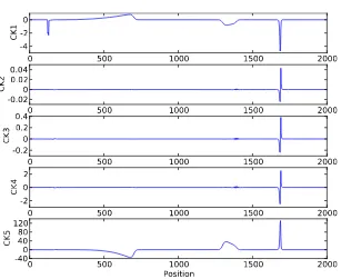
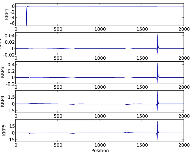
1500) are given initially. Here the spatial domain is discretized into 800 cells uniformly.Recall that from the previous sections, the weak local residual of the mass conservation with linearB-splines as the test function leads to the cheapest computation in comparison to the other formulation of the residuals. Interestingly, we find that the weak local residual of the mass conservation performs the best among others. This residual gives detection of the shock (which occurs in the dam break simulation) much clearer than the others. That is shown in our results inFigs. 1–3. Here CK1, CK2, CK3, CK4 and CK5 mean Constantin–Kurganov indicators(9)for the conservation laws listed inTable 1
respectively. Similarly KKP1, KKP2, KKP3, KKP4 and KKP5 mean Karni–Kurganov–Petrova indicators(6)for the conservation laws listed inTable 1respectively.
Fig. 1. Simulation results of the dam break problem at timet=20.
Fig. 2. The CK indicators for the dam break problem at timet=20.
We see the water surface (stage), momentum and velocity at timet
=
20 inFig. 1. A wet/dry interface moves to the left on the half left part of the domain, while a shock propagates to the right on the half right part. A good smoothness indicator must detect the shock by providing larger values of residuals at the shock position than at other smoother regions.The corresponding weak local residuals of the first five conservation laws using linearB-splines as the test function are shown inFig. 2. All residuals detect the shock. The residuals based on the second, third, fourth, and fifth conservation laws perform similarly. However, the residual based on the second conservation law gives the most obvious difference between the smooth and nonsmooth regions. The residual CK1 based on the first conservation law also detects the wet/dry interface, but it is correct in theory, as the first conservation law conserves the velocityu. Note that even though the wet/dry interface is a smooth transition with respect to water heighthand momentumuh, it is actually a discontinuity with respect to velocity
[image:4.544.123.430.301.552.2]Fig. 3. The KKP indicators for the dam break problem at timet=20.
The corresponding residuals of the first five conservation laws using quadraticB-splines as the test function are shown in
Fig. 3. All residuals are successful as smoothness indicators, except the residual based on the first conservation law. The resid-ual KKP1 based on the first conservation law does not detect the shock. Instead of detecting the shock, it detects only the mov-ing wet/dry interface by producmov-ing larger values of residuals at this wet/dry interface than at other positions on the domain. As follows, we explain why the residuals CK1 and KKP1, which are based on the first conservation law, generate large indicator values at the moving wet/dry interface. The velocityuis computed using the formulau
=
uh/
h. The wet area around the wet/dry interface has smallh. Consequently the velocityuis large at this wet area. Note that the velocityuis zero at dry areas. Therefore the moving wet/dry interface in the dam break problem has a large jump discontinuity in velocity, as shown inFig. 1. As a result, residuals based on the velocity conservation equation (the first conservation law) generate large indicator values at the wet/dry interface. The larger jump discontinuity leads to the larger residual. In addition, we note that the larger support size of the test function results in more number of cells and more number of time steps being involved in residual computations. Therefore, the residuals based on the velocity conservation equation at the wet/dry interface can dominate the indicator values over the whole domain, when the test function involved in the formulation has a large support size. This is demonstrated by KKP1 inFig. 3.5. Conclusion
Some weak local residuals relating to the shallow water equations have been investigated. We find that the weak local residual of the mass conservation law using linearB-splines as the test function is the best in terms of its ability to detect the smoothness of numerical solutions and in terms of its computational cost. Therefore, even though the shallow water equations admit infinitely many conservation laws, there is no need to use more complicated conservation laws of these equations when we want to detect the smoothness of solutions. Furthermore, we claim that weak local residuals can still be used as smoothness indicators for the shallow water equations with source terms. This is true as long as computations of weak local residuals are well-balanced with respect to the source terms. If they are not well-balanced, then it is possible to obtain nonzero weak local residuals when we simulate the steady state of a-lake-at-rest. We shall discuss ‘‘well-balanced computations of weak local residuals for the shallow water equations’’ in detail in a separate paper.
References
[1]S. Karni, A. Kurganov, G. Petrova, A smoothness indicator for adaptive algorithms for hyperbolic systems, J. Comput. Phys. 178 (2002) 323–341. [2]S. Karni, A. Kurganov, Local error analysis for approximate solutions of hyperbolic conservation laws, Adv. Comput. Math. 22 (2005) 79–99. [3]G.B. Whitham, Linear and Nonlinear Waves, John Wiley & Sons, New York, 1999.
[4]L.A. Constantin, A. Kurganov, Adaptive central-upwind schemes for hyperbolic systems of conservation laws, in: F. Asakura, et al. (Eds.), Hyperbolic Problems: Theory, Numerics, and Applications, Proceedings of the 10th International Conference, Osaka, Japan, 13–17 September 2004, vol. 1, Yokohama Publishers, Yokohama, 2006, pp. 95–103.