THE IMPACT OF LARGE URBAN STRUCTURAL ELEMENTS ON TRAFFIC FLOW
- A CASE STUDY OF DANWEI AND XIAOQU IN SHANGHAI
H. Lyu a*, L. Ding ab, H. Fan c, L. Meng a
a
TUM, Chair of Cartography, TUM, 80333 Munich, Germany- (hao.lyu, linfang.ding, liqiu.meng)@tum.de b Group of Applied Geoinformatics, University of Augsburg, 86159 Augsburg, Germany
c
Geographisches Institut, Universität Heidelberg, 69120 Heidelberg, Germany - [email protected]
Commission IV, WG IV/3
KEY WORDS: Danwei and Xiaoqu, road network, betweenness centrality, floating car data, traffic flow
ABSTRACT:
Danwei (working unit) and Xiaoqu (residential community) are two typical and unique structural urban elements in China. The interior roads of Danwei and Xiaoqu are usually not accessible for the public. Recently, there is a call for opening these interior roads to the public to improve road network structure and optimize traffic flow. In this paper we investigate the impact of Danwei and Xiaoqu on their neighbouring traffic quantitatively. By taking into consideration of origins and destinations (ODs) distributions and route selection behaviours (e.g., shortest paths), we propose an extended betweenness centrality to investigate the traffic flow in two scenarios 1) the interior roads of Danwei and Xiaoqu are excluded from urban road network, 2) the interior roads are integrated into road network. A Danwei and a Xiaoqu in Shanghai are used as the study area. The preliminary results show the feasibility of our extended betweenness centrality in investigating the traffic flow patterns and reveal the quantitative changes of the traffic flow after opening interior roads.
*
Corresponding author
1. INTRODUCTION
The Danwei (working unit) and Xiaoqu (residential community) are two typical and unique urban structure elements in China because of their distinctive cultural heritage and Chinese unique socialist background. The Danwei system was an important element of urban spatial structure in China. Danwei provides not only a working place, but also a comprehensive package for its staffs of daily life welfare and services, including residential buildings, canteen and shops. Some large Danwei even have their movie theatre, hospital and schools. Normally Danwei holds its facilities within its own territory with physical boundaries to prevent outsiders coming in in a disturbing manner. During the transition period Danwei is not being extinct, instead it was reformed into a new work-live balanced framework. In 1978, nearly 95% of the urban workforce was Danwei employees (Bray 2005), and most of them lived in Danwei compounds which constituted their daily-life circles. In 2004, there were still nearly 65% of city residents continued to reside in Danwei-based communities (Feng et al. 2004). Since mid-1980s with the trend of turning residential buildings from social welfare items to commodities, another concept, the so called ‘community’, has been developed (Bray 2006). In late 2000 Chinese Ministry of Civil Affairs defined ‘community’ as ‘a social collective formed by people who reside within a defined and bounded district’ (Ministry of Civil Affairs of P. R. China 2000). The territory of the community is designated as ‘the area under the jurisdiction of the enlarged Residents’ Committee’. This points out that both Danwei and Xiaoqu share common physical characteristics: enclosure boundaries, inner facilities and buildings, and interior roads. Recently there is a call for opening these interior roads to the public to reduce traffic congestion and balance the traffic flow. However, there is
still a lack of study to indicate how much change will happen to current traffic patterns. In this work we initiate a set of discussions on how and to what extent the change of a road network (i.e., adding interior roads to the public road network) will affect the traffic flow in its neighbouring area. The key idea is to find out indicators that can be derived from the physical configuration of a road network, and their correlations with traffic patterns, so that the change of traffic flow can be inferred from the change of the physical configuration. In this work, we choose a typical Danwei and Xiaoqu and their neighbouring road network in Shanghai as our study area. Betweenness centrality as a popular space syntax metric is investigated in our study. We explain the advantages and disadvantages using betweenness centrality in investigating traffic patterns. In addition, we use a small amount of GPS enabled taxi trajectory data, one type of floating car data (FCD), to investigate real world traffic patterns in the study area.
2. REVIEW ON USING SPACE SYNTAX TO EXPLORING TRAFFIC PATTERNS
Space syntax was first proposed by Bill Hillier and Julienne Hanson (Hillier 1976, Hillier & Hanson 1984) as a tool to understand urban spatial organization patterns. Space syntax introduced a set of concepts to turn a study space into graph. Centrality metrics are revealed to be crucial to characterize structural properties of complex graphs (Freeman 1978, Freeman et al, 1991, Newman 2005). These metrics are frequently applied in studying urban transportations (Holme 2003 Borgatti 2005, Crucitti et al, 2006). The ‘space syntax’ community believes that the configuration of a city’s road network plays an important role in shaping urban mobility patterns (Hillier et al, 1993, Penn et al, 1998). Axial map is one of the most important concepts in space syntax. It consists of a minimal set of axial lines covering all the convex spaces and their connections to represent perceivable roads and their surrounding environment. Researches like (Hillier et al, 1993) suggest axial lines capture some portions on how visibility and freedom of movement influence human behaviour in spatial systems.
Since motor vehicles are restricted on road networks, many researches choose to perform analysis directly on road networks other than derived axial maps. Road-centre line is an easily available representation for road network and can potentially serve as a bridge to connect space syntax and road network. Turner (2005) noticed that road-centre lines are broken across junctions, and therefore graph measures of the corresponding road-centre networks tend to vary with physical distance rather than the changes of direction as measured within axial networks. He introduced an angular segment analysis method to avoid the negative effects on graph measures. In addition, Thomson and Richardson (1999) proposed a stroke-based representation for road network from the observation that the angle of a turn has much impact on how human perceives the world. Later Thomson (2004) showed some advantages of using ‘strokes’ in road network analysis compare to using axial lines. A stroke is a linear, non-branching and connected chain aggregated from road segments according to continuity of direction, i.e. a minimum deflection angle within a certain value. Jiang and Claramunt (2004) argued that the naming system of a road network somehow reflects the public perceived image of the road network. In their paper, roads are merged from road segments of the same name. Later, Jang and his colleagues (Jiang et al. 2008) found the self-organized nature of urban roads and extended the idea ‘stroke’ road to ‘natural road’ based on the Gestalt principle of ‘good continuity’. They claimed that natural road network captures several essential characters of geographic space and navigation at human perception level. They examined correlations between 7 metrics and traffic patterns in the city of Gävle, Sweden.
The structural properties of a road network can be represented in both topological and geographic metrical forms. Geographic metrical representation is how road networks are usually modelled. In this form, a road network is abstracted as a graph, junctions as nodes and road segments as edges. Usually the road length between two junctions is marked as edge weight. Applying Poincaré duality to a geometric representation of a road network will generate a topological representation that road segments or roads are abstracted as nodes and their connections are indicated by junctions; the connections among each road segment nodes (road nodes) are denoted as edges. In topological representations geometric information like distance and location is omitted while the connectivity is preserved.
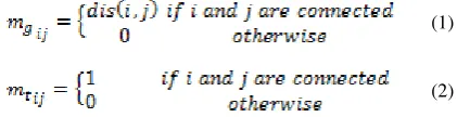
Figure 1 depicts exemplary road networks, with the form of road segments (Figure 1. a) and natural roads (Figure 1. b) and the respective corresponding topological representations. In a matrix manner, geographic representation can be written as matrix . Its element is the distance between
junction i and junction j if the two junctions is connected by a road segment, and 0 otherwise (as Formula 1). In topological representation matrix , its element is 1 if road
segment i and road segment j are intersected at some junction points, and 0 otherwise (Formula 2).
Figure 1. An exemplary road network a) in road segment form with corresponding topological representation, b) in natural road form with its topological representation (Jiang et al. 2008).
(1)
(2)
There is a wide spectrum of opinions on choosing metrics to explore urban traffic patterns. The most used ones include connectivity, integration, betweenness centrality, closeness and page ranking, and etc. (Hillier et al. 1993, Jiang & Claramunt 2004, Jiang et al. 2008, Jiang & Liu 2009, Kazerani & Winter 2009). Jiang (2009) provides a formal description for these three types of metrics. Based on the concept of depth, traditional space syntax metrics including connectivity, local integration, and global integration can be presented uniformly by counting linkage number in depth-wise from local to global. Another type of metrics, clustering coefficient, is defined by the probability of two neighbours of a given node that are linked together, and is measured by a ratio of actual links to all possible links, among the neighbours of the given node (Watts & Strogatz1998). Betweenness centrality is one of such metrics. Aside from the two mentioned types, PageRank metric, originally used by Google Search for ranking an individual web page, is also borrowed to explore traffic patterns.
3. BETWEENNESS CENTRALITY AND TRAFFIC PATTERNS IN NEIGHBOURING AREA
Betweenness centrality is selected in our study to bridge physical configuration of road network and traffic flow. Original definition of betweenness centrality is based on the idea that a node is more central when it is traversed by a larger number of the shortest paths connecting all pairs of nodes in the network. The betweenness centrality of a node v is given by the expression:
where = the total number of shortest paths from node to node
= the number of all those paths that pass through node
Betweenness centrality of an edge can be calculated in a similar way by counting how many times the edge is used by all possible paths over the total number of these paths. Usually the total number of possible paths is fixed, so we only use the counts for each edge. The definition of betweenness centrality assumes that Origins-Destinations (ODs) are evenly distributed among junction (or road segments) nodes, and people always choose geographic (or topological) shortest paths.
However, betweenness centrality is unsuitable to be applied directly to investigate traffic flow in a neighbouring area. Its original definition takes the whole road network into account, while a neighbouring area is only a patch. All possible paths in the whole road network can be divided into three categories: 1) the entire path falls in the neighbouring area, 2) part of the path falls into the neighbouring area, 3) the path never runs into the neighbouring area. When betweenness values are calculated with the original definition for a neighbouring area, only the first category paths are taken into account. Thus a road segment that is passed by several paths belonging to all three categories is down rated while a road segment that is passed only by the first category is up rated. The road segments near the border of a neighbouring area particularly suffer from such a problem. Even when the road segment is very important in the whole road network, the calculated betweenness value could be very small or even zero. As illustrated in Figure 2 and Table 1, the calculated shortest paths for the entire road network and the cutted neighbouring road network are of huge differences, which will result in different betweeness values.
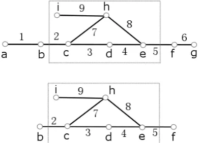
Including or excluding some road segments in a road network will change all betweenness values. This change comes from two facts according to the original definition of betweenness centrality. Firstly, it changes the OD distribution in the road network; secondly, it affects the shortest paths by bring in either new short cuts or detours. The example road network (in Figure 3. a) that consists of 5 natural roads illustrates this case. After closing (or removing) road C from the original road network, the resulting new road network could be like Figure 3(b). Their topological representations are illustrated in Figure 3(c) and (d) correspondingly. In Table 2, betweenness value is calculated for each road under two different scenarios, i.e. road C is open and road C is closed. The change of betweenness centrality is listed in Table 2. It shows a significant effect to the whole road network when road C is shut down.
Figure 2. The illustrative road network (up) and a neighbouring area of it (bottom).
Table 1. Counts of shortest paths that passes node and edge (any distinct unordered nodes pair has one path) for entire road
network (ERN) and for a neighbouring area (NA) of the illustrative road network in Figure 2.
Figure 3. a) an example road network, b) the road network when road C is excluded, c) topological representation of the road network when road C is included, d) topological representation
of the road network when road C is excluded.
In order to estimate the change of traffic patterns in the neighbouring area after opening interior roads, we need to extend betweenness centrality. Urban traffic patterns can be viewed as a collection of individual travel behaviour. As Gao and his colleagues (Gao et al. 2013) pointed out that betweenness centrality and real world traffic data could be mismatch since there are also complex human and geographic factors. In our study we extend betweenness centrality with unevenly distributed ODs and more complicated route selection behaviours.
Table 2. Betweenness values and the changes of the values.
Several studies imply that the distribution of origins and destinations varies in different area over entire city. Ding and her colleagues (Ding et al, 2015, Ding 2016, Jahnke et al, 2017) studied traveling behaviour of taxi-drivers from both individual
level and statistical level. They spot several ‘hot spot’ such as traffic hubs and functional areas, where there are more taxis travel through. Figure 4 and 5 show individual taxi data and 100 OD samples in Shanghai, China. (Both figures are from Ding 2016) We use Monte Carlo simulation to generate all possible OD pairs in the neighbouring area, and tune the number of ODs with consideration of all three paths categories. We consider impacts of crossings and road capacity to on route selection and extend the shortest path to the least cost path.
Figure 4. GPS samples of one taxi in one day, dots in red means the taxi is occupied, blue dots indicate non-occupied.
Figure 5. OD lines for100 taxi GPS samples
In GPS enabled navigation systems, the shortest path algorithm plays a fundamental role in routing function. However, drivers do not always want to follow topologically or geometrically shortest paths. Researchers put much effort to learn the needs from different drivers and try to provide them personalized navigation and way-finding solutions. For example, Krisp and Keler (2015) try to provide routes with less complicated crossings for inexperienced drivers. Jiang et al. (2008) also argue that crossings and turning angles may be important in road network organization and human path selection behaviour. We intend to assign some costs to a path when it passes a crossing and turns at a crossing. We use a piecewise function to simply empirically estimate additional costs of crossings and turning angles along a path. For example, when a path passes a crossing point and the turning angle is between -60 degree to 60 degrees, we assign additional 10 units of costs to the path. Similarly, when the turning angle is in (60, 120) or (-60, -120), 20 units of costs is added, and if the turning angle greater than 120 degree or less than -120 degree, 30 units of costs is added. Road capacity is another important consideration when selecting routes. Usually, the increased number of vehicles indicate the reduced travelling speed and the longer waiting time at crossings. Routing between all OD pairs is required to be an accumulative process. When more paths go through certain road segments, additional capacity penalties are added, according to its capacity and the number of path count. This prevents any road segment from being unreasonably visited by too many paths. After the penalty reaches a certain value w.r.t. the road segment’s capacity (e.g., character by number of lanes, length), some paths that use this road segment will randomly make a detour with less crowded roads.
4. A CASE STUDY IN SHANGHAI
4.1 A Brief Introduction of Study Area
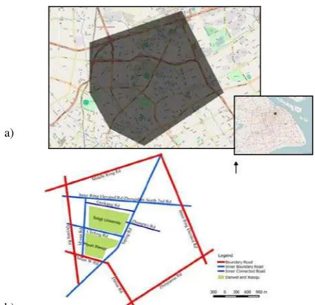
The study area is part of Shanghai, China, and contains a Danwei, i.e. Tongji University and a Xiaoqu, named as Miyun Xiaoqu (as Figure 6. a). The study area is roughly bounded by 6 main roads: Quyang Road on the west, Inner Ring Elevated Road (Zhongshan North 2nd Road) on the north and partly on the east, Zoujiazui Road on the east and Dalian West Road and Dalian Road on the west. Siping Road is the longest road across the whole study area. Tonji University is a typical Danwei in Shanghai, its campus area is bounded by Miyun Road in west, Chifeng Road in south, Siping Road in east and Inner Ring Elevated Road in north. South of Tongji University is a Xiaoqu named Miyun Xiaoqu. There are dense interior roads in the campus area. However, these roads are not accessible for the public who does not work or live there. We sketch these roads in Figure 6. b.
The road network data of Shanghai is represented by road central lines. All road segments are bi-direction accessible and there is no one-way road in the study area. Roads inside Danwei and Xiaoqu are taken from OpenStreetMap (OSM) dataset1. Some missing roads are added manually. To assess the impact of the closure of Danwei and Xiaoqu on their surrounding area, we consider two scenarios in the road network. In the first scenario (Figure 7. a), the interior roads of Danwei and Xiaoqu are not accessible and marked as background roads in colour grey. They are not used in betweenness calculation in this case. In the second scenario, interior roads of Danwei and Xiaoqu are accessible and marked in solid black line as neighbouring public roads (Figure 7. b). In this scenario, interior roads are used in betweenness calculation, while they are not involved in generating OD pairs.
Figure 6 a) Study area in Shanghai, China. Study area is covered by a light grey shadow. Open Street Map (OSM) is
used as base map, b) Sketch map for study area
In our study, we first show the shortages of using original betweenness definition and then calculate extended betweenness values. We assume a stable OD distribution no
1
The mentioned part of map data copyrighted OpenStreetMap contributors and available from https://www.openstreetmap.org
a)
matter interior roads are included or excluded. Crossing penalty and capacity penalty are considered as two additional sources of cost in the routing algorithm. Our method does not require to merge road segments into named streets or natural roads (Jiang et al. 2008), and we keep the original spatial structures of road network.
Figure 7. Neighbouring road network for the study area: a) without interior roads of Danwei and Xiaoqu and, b) with
interior roads of Danwei and Xiaoqu.
Figure 8 is an overview of original betweenness values in study area. These values are normalized and colour coded from blue to red to indicate the increasing betwenness values. Before integrating the interior roads of Danwei and Xiaoqu, Siping Road has the highest betweenness value, followed by Miyun Road and Inner Ring Elevated Road/Zhongshan North 2nd Road. Zhangwu Road, Chifeng Road and Guokang Road have rather low betweenness values. After the integration, betweenness values of Chifeng Road and Guokang Road are significantly increased, and the betweenness value of Zhangwu Road is also slightly increased.
Figure 8. Betweenness centrality values calculated by original definition, a) when interior roads of Danwei and Xiaoqu are not
integrated into the road network, b) when interior roads of Danwei and Xiaoqu are integrated into the road network
Figure 9. Betweenness centrality values calculated by simulation, a) when interior roads of Danwei and Xiaoqu are not integrated into the road network, b) when interior roads of Danwei and Xiaoqu are integrated into the road network.
As discussed in section 3, when only consider paths that entirely fall into study area, Siping Road, which goes across the study area from the north to the south gains more scores at the middle part, while boundary roads such as Middle Ring road gain less scores. However, Middle Ring Road is actually an
important city express road in Shanghai. From Figure 8 b, we can see that integrating interior roads to public road network even reinforces this phenomenon and attracts the high betweenness value close to these roads. On one hand, the newly added roads introduces new possible paths in the road network when calculating betweenness values, on the other hand it changes the original OD distribution.
Figure 9. a and b show betweenness centrality values that calculated by randomly generated 20000 ODs in the study area with a uniform distribution over all nodes. The betweenness centrality values are similar to the values calculated by the original ones, while it down rates road segments that have less least cost paths passing through (compare Figure 8. a and Figure 9. a, Figure 9. b, see road segments in the left part). When interior roads are integrated into the public road network, it does not dramatically change extended betweenness centrality patterns (compare Figure 9. a, and b), which means interior roads are seldom selected in terms of least cost paths.
4.2 Traffic flow in study area
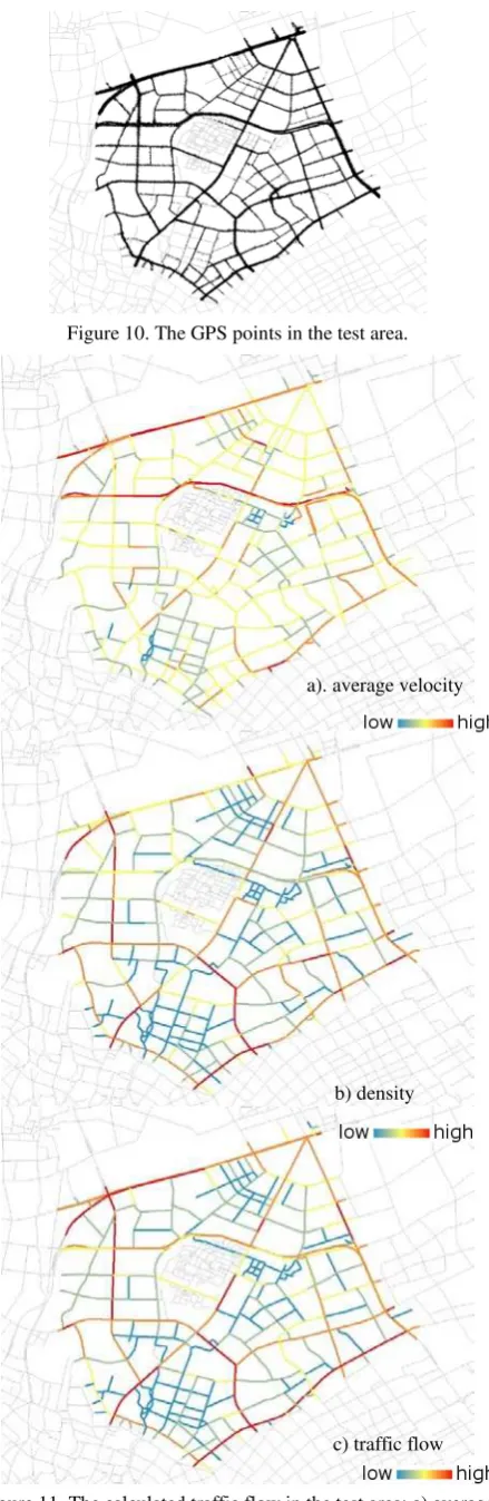
Floating taxi car data is used to examine how betweenness centrality reveals the real world traffic flow. The test data are temporally ordered position records collected from about 2000 GPS-enabled taxis on 18th May 2010, in Shanghai. The temporal resolution of the dataset is 10 seconds and thus theoretically around 8000 GPS points of each car would be recorded in one day (24 hours) given the GPS device effective. Each position record has nine attributes, i.e. car identification number, company name, current timestamp, current location (longitude, latitude), instantaneous velocity, and the GPS effectiveness. Detailed description of these fields is in Table 3. In our work, we extract the GPS records in the test area around Tongji University and exclude the records of low velocity, e.g. v<5km/h, which results in about 156,600 records. Figure 8 shows the extracted GPS points in the test area.
According to the general traffic flow models (Gerlough & Huber 1975), we adopt the formula 4 to calculate the traffic flow:
(4)
where f= traffic flow d = vehicle density v = average velocity
and are calculated based on a buffer of 30m for each street. Figure 11 illustrates the respective results.
Field Example field value
Field description
Date 20100517 8-digit number, yyyymmdd Time 235903 6-digit number, HHMMSS Company name QS 2-digit letter
Car identifier 10003 5-digit number
Longitude 121.472038 Accurate to 6 decimal places, in degrees
Latitude 31.236135 Accurate to 6 decimal places, in degrees
Velocity 16.1 In km/h
Car status 1/0 1-occupied; 0-unoccupied GPS effectiveness 1/0 1-GPS effective; 0-ineffective
Table 3. Description of the fields of floating car data. b)
a)
a) b)
Figure 10. The GPS points in the test area.
Figure 11. The calculated traffic flow in the test area: a) average velocity b) traffic density c) traffic flow (best viewed in colour)
As Figure 11 depicts, there is a high correlation between traffic density and traffic flow. The main roads of the study area all have high traffic flows, e.g., Inner Ring Elevated Road/Zhongshan North 2nd Road, Siping Road, Quyang Road, and Zhoujiazui Road. Road segments that connects main road have relatively lower traffic flows. The short branches scattered in the study area have the lowest traffic flow values. When comparing Figure 8. a, Figure 9. a, and Figure 11, one may find out that calculating betweenness centrality without considering OD distributions and path selection behaviours cannot reflect real traffic patterns in study area.
4.3 Extended betweenness centrality and traffic flow
In our experiment we simulated OD pairs over all study area, every node of road segments can be potential origin/destination points. We carefully adjust the appearance frequency of certain OD pairs so that the calculated results can approximate the traffic flow in this area. It should be noticed that the generated OD pairs can be very different from the real OD distribution. It is meaningless to discuss an OD pair and the path between them in our simulation, we only discuss the results as a whole. Figure 13 gives one simulation result to generate 10000 OD pairs, the line width and colour all each indicates the counts of the same OD pairs. Thicker line or darker colour means more repetition. The appearance counts of different OD pairs can vary from 1 to more than 750 times out of 10000. Most generated OD pairs are located on the boundary of study area. We can expect paths between these OD pairs also pass through this area. There are also minor OD pairs fall in the inner part of the study area. The result also meets our hypothesis that quite a number of paths with ODs outside the study area should be considered in order to approximate the real traffic.
The extended betweenness centrality calculated with the same 10000 ODs are shown in Figure 13. They have a certain correlation (R square values 0.9) with real world traffic flow patterns.
Figure 12. 10000 simulated ODs to approximate traffic flow in study area
After including interior roads of Danwei and Xiaoqu into public road network, we keep the ODs generated from the first scenario. Then these ODs are used to generate new paths on the changed road network. The calculated betweenness values are given in Figure 14, colour ramp from blue to red indicate betweenness values from low to high. In both calculations we generate 10000 paths, so there is no need to do normalization and we can compare these values directly. In Figure 14, we only observe little change happened to traffic patterns in study area. Most traffic flows are still distributed on main roads, similar a). average velocity
b) density
with real traffic flow as we mentioned in section 4.2. One difference we find directly from visualized result is that an observable pattern changes on Quyang Road. As Quyang Road has a high vehicle density some of the paths that pass Quyang Road tried a detour on Miyun Road.
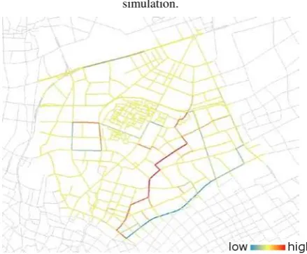
Figure 13. Extended betweenness centrality values with the generated ODs in Figure 12.
Figure 14. Simulated betweenness centrality values after integrate interior roads, with the same ODs as in previous
simulation.
Figure 15. Difference simulated betweenness value between before and after the integration of interior roads into public road
network.
When taking a closer look at specific value changes in Figure 15, most of simulated betweenness values remain unchanged, and drastic changes happened on several road segments, for example on Zoujiazui Road and some branch roads. Before integrate interior roads, there is about 500 path counts on Zoujiazui Road. In Figure 14, blue extreme colour represents a changed value of -170 counts, while the red extreme colour represents a changed value up to 140, and yellow colour in the middle of the colour ramp represent 0. Except these drastic changes, traffic flow patterns also slightly change on some roads around Danwei and Xiaoqu. For example, Chifeng Road and part of Siping Road (from crossing with Chifang Road and the entrance of interior roads in Tongji Univercity) the path counts changes slightly as -40. Before integrate interior roads, path counts of these two roads are about 160 and 400. Other roads around Danwei and Xiaoqu has no significant change in traffic flow (between ±10).
5. CONCLUSION
In this paper we focused on how Danwei and Xiaoqu, two typical enclosed large urban structural units in China, affect their surrounding traffic patterns. It may be a common sense that if the interior roads were open to the public the surrounding traffic load should be eased. We performed a quantitative analysis to investigate how traffic flow will be changed if interior roads are opened to the public. The analyse of traffic flow change was performed in two scenarios. The first one is a real world scenario in which interior roads of Danwei and Xiaoqu are not accessible for the public and excluded from urban road network. In the other scenario we assumed that the interior roads of Danwei and Xiaoqu are accessible for the public, and are integrated into the urban road network. Floating car data from taxis are used to find out how much our analysis close to the real world traffic patterns.
In the analysis we use betweenness centrality as a bridge to characterize traffic patterns. In order to apply betweenness analysis to a neibhbouring area, we modified its original definition from a probabilistic perspective. ODs that outside study area is simulated by Monte Carlo method. Besides, we also extended the ‘shortest path’ in original betweenness definition to ‘least cost path’ to fit our intuition on route selection behaviours. The extended betweenness centrality has certain correlation with traffic flow and shows reasonable similarity with the real world traffic flow.
The simulated results show the closure of Danwei and Xiaoqu affects their surrounding roads by increasing their traffic flow volumes. On the contrary, an open roads system in Danwei and Xiaoqu could lead to a more balanced traffic flow, and ease the tension of high traffic density. Despite the economic and social perspectives that usually used by human geographers, we explored Danwe and Xiaoqu from a different perspective with the focus on traffic. We hope our work will contribute to the evolution of Danwei and Xiaoqu, for achieving a balanced status on their enclosed social structure and openness of the public traffic accessibility.
ACKNOWLEDGEMENTS
We sincerely thank Prof. Chun LIU from Tongji University, Shanghai, for sharing with us the Floating car data. The first author also appreciates the financial support from China scholarship council (CSC) for his PhD study.
REFERENCES
Borgatti, S. P. (2005). Centrality and network flow. Social networks, 27(1), 55-71.
Bray D (2005). Social space and governance in urban China: The danwei system from origins to reform. Stanford University Press.
Bray D (2006) Building ‘community’: new strategies of governance in urban China. Economy and Society 35(4): 530-549.
Crucitti, P., Latora, V., & Porta, S. (2006). Centrality in networks of urban streets. Chaos: an interdisciplinary journal of nonlinear science, 16(1), 015113.
Ding, L. 2016. Visual Analysis of Large Floating Car Data - A Bridge-Maker between Thematic Mapping and Scientific Visualization, Doctoral Thesis, Technical University of Munich
Ding, L., Yang, J., & Meng, L. (2015). Visual Analytics for Understanding Traffic Flows of Transport Hubs from Movement Data. In Proc. International Cartographic Conference, Rio de Janeiro, Brazil, Aug (pp. 23-28).
Feng J, Zhou Y, Wang X and Chen Y (2004) The development of suburbanization of Beijing and its countermeasures in the 1990s. Planning Study 28(3): 13-29.
Freeman, L. C. (1978). Centrality in social networks conceptual clarification. Social networks, 1(3), 215-239.
Freeman, L. C., Borgatti, S. P., & White, D. R. (1991). Centrality in valued graphs: A measure of betweenness based on network flow. Social networks, 13(2), 141-154.
Gao S, Wang Y, Gao Y and Liu Y (2013) Understanding urban traffic-flow characteristics: a rethinking of betweenness centrality. Environment and Planning B: Planning and Design 40(1): 135-153.
Gerlough D and Huber M (1975) Traffic flow theory. Washington DC: Special Report 165. Transportation Research Board.
Hillier, B., Leaman, A., Stansall, P., & Bedford, M. (1976). Space syntax. Environment and Planning B: Planning and Design, 3 (2), 147-185.
Hillier B and Hanson J (1984). The social logic of space. Cambridge university press.
Hillier B, Penn A, Hanson J, Grajewski T and Xu J (1993) Natural movement-or, configuration and attraction in urban pedestrian movement. Environment and Planning B: Planning and Design 20(1): 29-66.
Holme, P. (2003). Congestion and centrality in traffic flow on complex networks. Advances in Complex Systems, 6(02), 163-176.
Jahnke, M., Ding, L., Karja, K., & Wang, S. (2017). Identifying Origin/Destination Hotspots in Floating Car Data for Visual Analysis of Traveling Behavior. In Progress in Location-Based Services 2016 (pp. 253-269). Springer International Publishing.
Jiang, B. (2009). Ranking spaces for predicting human movement in an urban environment. International Journal of Geographical Information Science, 23(7), 823-837.
Jiang B and Claramunt C (2004) Topological analysis of urban street networks. Environment and Planning B: Planning and Design 31(1): 151-162.
Jiang B and Liu C (2009) Street ‐based topological representations and analyses for predicting traffic flow in GIS. International Journal of Geographical Information Science 23(9): 1119-1137.
Jiang B, Zhao S and Yin J (2008) Self-organized natural roads for predicting traffic flow: a sensitivity study. Journal of
statistical mechanics: Theory and experiment 2008(07):
P07008.
Kazerani A and Winter S (2009) Can betweenness centrality explain traffic flow. In: Proceedings of the 12th AGILE International Conference on GIS.
Krisp, J. M., and Keler, A. (2015). Car navigation–computing routes that avoid complicated crossings. International Journal of Geographical Information Science, 29(11), 1988-2000.
Ministry of Civil Affairs of P. R. China (2000) ''Minzhengbu' guanyu zai quanguo tuijin chengshi shequ jianshede yijian' (The Ministry of Civil Affairs' views on promoting urban community building throughout the nation'). Ministry of Civil Affairs of P. R. China. Beijing, Minzhengbu.
Newman, M. E. (2005). A measure of betweenness centrality based on random walks. Social networks, 27(1), 39-54.
Penn, A., Hillier, B., Banister, D., and Xu, J. (1998). Configurational modelling of urban movement networks. Environment and Planning B: planning and design, 25(1), 59-84.
Thomson R C and Richardson D E (1999) The ‘good continuation’ principle of perceptual organization applied to the generalization of road networks. In: Proceedings of the 19th International Cartographic Conference, Ottawa, Canada, pp. 1215-1223
Thomson R C (2004) Bending the axial line: Smoothly continuous road centre-line segments as a basis for road network analysis. In: Proceedings 4th International Space Syntax Symposium, London, UK.
Turner A (2005) Could a road-centre line be an axial line in disguise. In: The 5th International Space Syntax Symposium, Delft, Netherlands.
Watts, D. J., and Strogatz, S. H. (1998). Collective dynamics of ‘small-world’ networks. nature, 393(6684), 440-442.