Volume 28, Number 1, 2013, 45 – 61
SPATIAL SMALL AREA ESTIMATION FOR DETERMINATION
OF UNDERDEVELOPED VILLAGES IN THE PROVINCE
OF YOGYAKARTA (DIY) IN 2011
1Lilis Nurul Husna
Badan Pusat Statistik (BPS) RI ([email protected])
Sarpono
Head of Standardization and Statistical Classification BPS RI ([email protected])
ABSTRACT
Indonesia's poverty alleviation programs are implemented by two approaches target, those are the pockets (areas) of poverty and the poor households. Related with poverty alleviation programs targeting poor areas, in the Medium Term Development Plan (RPJM) 2010-2014, the government through the Development Backward Areas Ministry (KPDT) has determined the backward or underdeveloped regions at the level of district/city. There is no district/city in the province of Yogyakarta (DIY) are classified as underdeveloped region, but in 2011 the poverty rate in DIY is the highest compared with other provinces in Java and Bali. Therefore, the classifications of underdeveloped areas are not optimal if applicable only within the district, but it needs to be seen in the smaller scope, such as village. The main purpose of this study is to determine the underdeveloped villages in DIY in 2011. The average per capita household expenditure is a key indicator in measuring poverty. Susenas data can only be used to estimate the average per capita household expenditure to the level of district. Therefore, to obtain the estimated value in village level, this study used Small Area Estimation approach by combining census data (Podes 2011) and survey data (Susenas 2011). This study used Geographically Weighted Regression (GWR) with Adaptive Gaussian Kernel Bandwidth weighting function. GWR is a linear regression model that produces the local parameters in all locations. GWR parameters estimated are performed by Weighted Least Squares (WLS) method which involving spatial aspects. The results found that there were 13 underdeveloped villages in DIY. Furthermore, the Local Indicator of Spatial Association (LISA) is used to look at the tendency of cluster in underdeveloped villages. Then, maps are used to compare charac-teristic of underdeveloped villages among others.
Keywords: poverty, underdeveloped areas, spatial, SAE, GWR
1
INTRODUCTION
Since early 1970s, poverty alleviation is a priority in Indonesia development strategies. The main objective of poverty reduction strat-egy is to improve the resident welfare and re-duce socio-economic disparities or inequality intergroup residents. Poverty alleviation pro-gram directly implemented in early 1990s. At that time, the government has formulated sev-eral programs targeted using two approaches, namely pockets (areas) of poverty and the poor households. Target areas refer to to the identification of poor or underdeveloped areas. Meanwhile, individual targets aimed at house-holds or residents who have low incomes (un-der the poverty line) (BPS, 2004).
Related with poverty alleviation programs which targeting poor areas, in the Medium Term Development Plan (RPJM) 2010-2014, the government through the Development Backward Areas Ministry (KPDT) has set the backward/underdeveloped regions based on six main criteria, those are: (1) economic soci-ety, (2) human resources, (3) infrastructure, (4) local financial capacity (fiscal gap), (5) accessibility, and (6) the area characteristics. In addition to these basic criteria, it is also considered that the condition of the district is located in the border areas between countries, disaster-prone areas, and areas otherwise specified.
Development of underdeveloped areas is a deliberate attempt to change a region occupied by communities with different socio-economic problems and physical limitations, to be de-veloped by the community whose have same quality or nearly same compared with other Indonesian society. Development of underde-veloped areas program focused on accelerating development in the areas of social, cultural, economic, financial areas, accessibility, and the infrastructure supplay is still lagging be-hind compared to other areas.
In the 2005-2009 Development Planning, there are two districts in the Province of Yogyakarta (DIY) included in underdeveloped areas, namely Gunung Kidul and Kulon Progo. In 2009, the two of them classified as the
ade-quate district so in 2010-2014 Development Planning, no districts in DIY is underdevel-oped area. Nevertheless, based on BPS, in 2011 DIY poverty level at is still in top of the rank in the Java-Bali, amounting to 16,08 per-cent, higher than Jakarta (3,75 percent), Bali (4,20 percent), Banten (6,32 percent), West Java (10,65 percent), East Java (14,23 per-cent), and Central Java (15,76 percent).
Based on these facts, classifications of un-derdeveloped areas are not optimal if only applicable within the district, but it needs to be seen more in the smaller scope, such as vil-lages. BPS has been several times determine underdeveloped villages, namely in 1993, 1994, and 2002. In 1993, BPS used 33 vari-ables. In 1994 BPS used 17 variables to urban areas and 18 variables rural areas. In 2002 BPS set the determination of underdeloped villages uses 19 variables for urban areas and 17 variables for the rural areas.
According to BPS (2005), underdeveloped villages are villages whose condition is rela-tively worse from other villages. Development of an area is reflected by the main indicators, namely the level of average per capita house-hold expenditure. The average per capita household expenditure can be obtained from the Susenas, but it can only be used to estimate in district level. Therefore, this study com-bines survey data (Susenas) and census data (Podes) to obtain an estimated value of village level, similar with the method developed by the World Bank in conducting small area es-timation (Hentschel, et al., 2000).
affected by location of the observation or the village, including the position of the other vil-lages around that (Rita & Anik, 2010). Thus, involving spatial factors are important in poverty analysis.
Based on that background, this study aims to determine underdeveloped villages in DIY by using local spatial regression models, namely Geographically Weighted Regression (GWR). Moveover, it also descibes the condi-tion of underdeveloped village in DIY. This study is expected to give benefit in reduce poverty efforts in DIY and inspire govern-ments and other researchers in the method of determining the underdeveloped villages.
DATA SOURCES
This study uses secondary data from Na-tional Socio-economic Survey (Susenas) 2011
and Villages Potential (Podes) 2011. The data was obtained from the BPS. The average per capita household expenditure got from Susenas is used as the response variable, while villages characteristics obtained from Podes used as predictor variables.
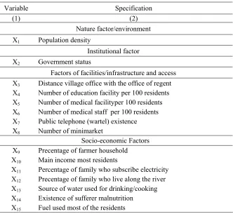
BPS (2005) determined that there are sev-eral factors suspected to be the cause of devel-opment of a village. They are natural tors/environmental, institutional factors, fac-tors of facilities/infrastructure and access, and socio-economic factors. Based on Podes 2011 availabel data, this study used 15 variables covering those four factors to remains under-developed village establish model as presented in Table 1.
Table 1. Predictor variables to determine underdeveloped village
Variable Specification (1) (2)
Nature factor/environment
X1 Population density
Institutional factor X2 Government status
Factors of facilities/infrastructure and access X3 Distance village office with the office of regent
X4 Number of education facility per 100 residents
X5 Number of medical facilityper 100 residents
X6 Number of medical staff per 100 residents
X7 Public telephone (wartel) existence
X8 Number of minimarket
Socio-economic Factors X9 Precentage of farmer household
X10 Main income most residents
X11 Percentage of family who subscribe electricity
X12 Precentage of family who live along the river
X13 Source of water used for drinking/cooking
X14 Existence of sufferer malnutrition
ANALYSIS METHOD
1. Global Regression Model
Global regression models that often used to examine the relationship between predictor variables and the response variable is a multi-ple linear regression with the model as fol-lowing: parameter values are estimated by Ordinary Least Square method (OLS) as follows:
y
Where X is the matrix variable predictor size
n x k, k is the number of parameters (k = p +1) and p is the number of predictor variables. The first column marik X is worth one. Mean-while, y is the response variable vector. In equation (1), the value of ˆ is assumed con-stant in all location so-called global model.
2. Geographically Weighted Regression (GWR)
Location produces two types of spatial ef-fects, those are spatial dependence and spatial heterogeneity (Anselin, 1992). Geographically Weighted Regression (GWR) is one method used to estimate the data that has a spatial het-erogeneity (Brunsdon, Fotheringham & Charlton, 1996). GWR will result local pa-rameter estimated, where each observation will have different parameter estimated. In GWR models, each observation is georefer-enced, which have coordinate points (latitude and longitude). The GWR model by Fother-ingham (2002) as follows:
i Where yi is the value of the dependent variable
in the i-th observations, xij is the value of the
j-th independent variable in the i-th observa-tion, β0(ui, vi) is intercept on the observations at-i, βj(ui, vi) is parameter estimated of predictor variable xj on i-th observation, p is the number of predictor variables, (ui,vi) is the coordinate points of observate location and εi is random error that assumed distributed
N(0, σ2I).
The parameters estimated by GWR mod-els will vary at all location, so there are nk
parameters to be estimated, which n is the
number of observation and k=p+1 is the number of parameters at each observation lo-cation. To estimate these parameters, GWR used Weighted Least Squares (WLS) method to give the differently weights at each obser-vation. In providing weighting, this method follows Tobler's First Law of Geography, which location that is near to the i-th location will have more effect in predicting the pa-rameters in i compared the further data. Thus, a nearer location will be given greater weighting.
Estimator for local regression coefficients in GWR are as follows: is a diagonal matrix with elements on that diagonals are geographical weighting on each location for observation location at-i, and other elements are zeros.
Where dij is the Euclidean distance between
i-th and j-th location and b is the bandwidth. Weighted value will be close to 1 if the dis-tance is near to the observation or coincide, and will become smaller so close to zero if the distance is farther away.
Determining the optimum bandwidth before forming the GWR models is very important (Fotteringham et al., 2002). One of methods can be used to determine the opti-mum bandwidth is the miniopti-mum Akaike Infor-mation Criterion (AIC). According Huvrich et al. (1998), AIC formula for GWR is as
Goodness of Fit Test needs to be done to see if the GWR models better than the OLS models. Testing is done as follows (Brunsdon,
et al., 1999): squared residuals OLS and GWR model. Model F will approach the F distribution with freedom degrees v12/v2, 12/2 where:
When the significance level is α, zero hipothesis stating that the GWR and OLS
models equally well in explaining the relation-ship between the predictor variables and the response variable will be rejected if F>Fα
( 2
Although the GWR main method used to explore the existence of spatial nonstationarity of the parameters, the prediction is an impor-tant aspect in the regression analysis. Predic-tion is done to get the value of the response variables in new areas, such as areas are not covered in the survey (Leung, et.al, 2000).
If the GWR model can explain well one set of data, then the model can be used to pre-dict the value of the variable response to a new location by using the predictor variables in the new location. Suppose
(
x x
01 02
x
0p)
is thevalue of the predictor variables at the new lo-cation (p0) and 0 (1 01 02... 0p) determined through model calibration process. Meanwhile, the distance between p0 with another point in the sample is also known if p0 coordinates are known.
3. Local Indicators of Spatial Association (LISA)
LISA is a statistical value used to test region propensity to experience the interaction region or outlier individually. LISA can be used to see the local spatial autocorrelation. Significant LISA values showed the village interacting with others significantly or an outlier.
j
j j ij i
i i
i i
i w x x
n x x
x x
I ( )
) (
) (
2 (13)
Where x is the mean of the x variable and wij is the weight matrix elements. The weights based on spatial boundaries, called the Queen Contiguity (side-angle intersection).
RESULTS
1. Poverty in the Province of Yogyakarta (DIY)
Poverty is a multidimensional problem. In macro, BPS uses basic needs approach. With
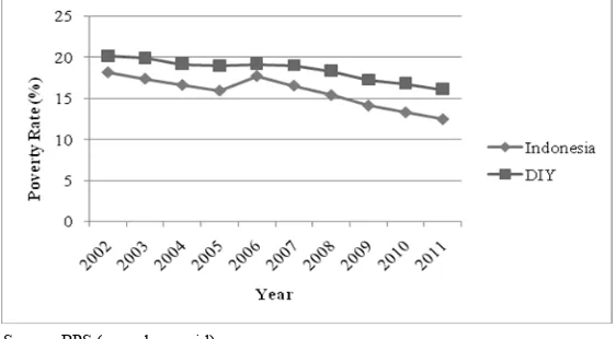
this approach, poverty is seen as an economic inability to meet basic needs of food and nonfood measured from the expenditure. In other words, the poor are people who have an average per capita expenditure per month under a line called Poverty Line (GK). Number of poor people in DIY in 2002-2011 can be seen in Figure 1.
Figure 1 shows that the level of poverty in DIY is always higher than the national average. When viewed in more detail, the percentage of poor people in each district in DIY can be described as illustrated in Figure 2.
Source: BPS (www.bps.go.id)
Figure 1. The poverty rate of DIY and Indonesia in 2002-2011
Source: BPS (Daerah Dalam Angka)
Figure 2 shows that in 2006 there was an increasing poverty rate in Kulonprogo, Gunung Kidul, and Bantul. This is occured because of the earthquake in DIY in 2006. Largest contributor to the poverty rate of DIY is Kulon Progo and Gunung Kidul. Thus, poverty reduction programs need to be focused on those two districts.
2. Parameter Estimated by GWR model
Brandon (2006) states that poverty is spatial problem. In analyzing spatial data, if spatial effects are ignored so the results of the analysis will be biased (Anselin and Griffith, 1988). Geographically Weighted Regression (GWR) is one of the most effective methods for estimating data that have spatial hetero-geneity (Brunsdon, et al., 1996).
Steps to build GWR models are presented in Figure 3.
Bandwidth
optimum
Weighting Function
Parameter Estimation
Hypothesis Testing START
STOP
Figure 3. Steps to build GWR models
Source: BPS (Susenas 2011, data proccesing with ArcGIS 10)
Determining the optimum bandwidth is based on the minimum AIC value 6579,80. This value is derived on the bandwidth 0,13 or 31 nearest villages from the observation. This study used adaptive bandwidth because the sampels of Susenas are not spread evenly (Figure 4). To obtain the weighting matrix, besides the bandwidth, Euclidean distance location (ui,vi) is also required for all sample locations. In this study, the Euclidean distance is measured from the center point between the villages with other villages. Equation (4) is used to obtain the estimated values of GWR parameters.
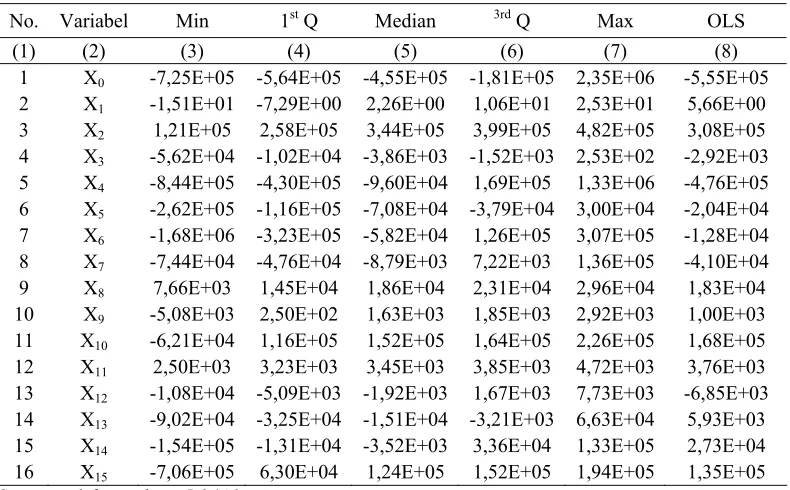
Table 2 shows the results of the parameter estimation of GWR and OLS models. GWR models will produce different parameter esti-mates at each location. Column 3 to column 7 consecutively shows descriptive statistics of the coefficients estimated by GWR models, namely the minimum, first quartile, median, third quartile, and maximum. Meanwhile, col-umn 8 shows the value of the coefficient
esti-mate OLS models is assumed to be constant at all locations.
Table 2 also providing information that GWR models can explain more phenomena than the OLS models that only produce one estimation parameter on each variable. For example, the relationship between population densities with an average per capita household expenditure can be positive or negative. Esti-mated value of the coefficient is positive, meaning that if there is an increase in the vil-lage population density, the average per capita household expenditure in the village will in-crease. It reflects that the population density increase in the village will increase welfare on that village. Meanwhile, the value of the coef-ficient estimated is negative which means that if there is population density increase in the village, the average per capita household ex-penditure in the village will decrease. It re-flects the population density increase of the village will not increase the welfare.
Table 2. Parameter estimated of GWR and OLS models
No. Variabel Min 1st Q Median 3rd Q Max OLS
(1) (2) (3) (4) (5) (6) (7) (8)
1 X0 -7,25E+05 -5,64E+05 -4,55E+05 -1,81E+05 2,35E+06 -5,55E+05
2 X1 -1,51E+01 -7,29E+00 2,26E+00 1,06E+01 2,53E+01 5,66E+00
3 X2 1,21E+05 2,58E+05 3,44E+05 3,99E+05 4,82E+05 3,08E+05
4 X3 -5,62E+04 -1,02E+04 -3,86E+03 -1,52E+03 2,53E+02 -2,92E+03
5 X4 -8,44E+05 -4,30E+05 -9,60E+04 1,69E+05 1,33E+06 -4,76E+05
6 X5 -2,62E+05 -1,16E+05 -7,08E+04 -3,79E+04 3,00E+04 -2,04E+04
7 X6 -1,68E+06 -3,23E+05 -5,82E+04 1,26E+05 3,07E+05 -1,28E+04
8 X7 -7,44E+04 -4,76E+04 -8,79E+03 7,22E+03 1,36E+05 -4,10E+04
9 X8 7,66E+03 1,45E+04 1,86E+04 2,31E+04 2,96E+04 1,83E+04
10 X9 -5,08E+03 2,50E+02 1,63E+03 1,85E+03 2,92E+03 1,00E+03
11 X10 -6,21E+04 1,16E+05 1,52E+05 1,64E+05 2,26E+05 1,68E+05
12 X11 2,50E+03 3,23E+03 3,45E+03 3,85E+03 4,72E+03 3,76E+03
13 X12 -1,08E+04 -5,09E+03 -1,92E+03 1,67E+03 7,73E+03 -6,85E+03
14 X13 -9,02E+04 -3,25E+04 -1,51E+04 -3,21E+03 6,63E+04 5,93E+03
15 X14 -1,54E+05 -1,31E+04 -3,52E+03 3,36E+04 1,33E+05 2,73E+04
16 X15 -7,06E+05 6,30E+04 1,24E+05 1,52E+05 1,94E+05 1,35E+05
These results support the research of Sumaryadi (1997) that population density may reflect different conditions of social welfare. Poor villages in urban areas are normally lo-cated in a sub-urban area with dense and ir-regular arrangement houses. Meanwhile, poor villages in the rural areas have low quality of human resources with sparse/less population density.
Coefficient estimates of GWR model for the variables of population density can be used to set the flow of population mobility. For example, village A populous and has negative coefficient estimated while village B sparsely populated and has a positive coefficient esti-mated. So, mobility can be directed from vil-lage A to vilvil-lage B, for example by opening new job vacancies in the area B. Thus, the development is expected to run optimally and evenly. Coefficient estimates of each village could be seen in Figure 6 (Appendix). In the meantime, in order to examine the relationship between response variable and predictor vari-ables at each location required other studies that are not included in this study.
GWR ability to capture spatial nonstation-arity should produce a better estimation than the global model. Some indicators can be used to compare global models and GWR model are smallest value of AIC, largest R2, smallest
ˆ and smallest Sum Square Residual (SSR). From Table 3 it can be seen that based on all the best model criterion, GWR model are better than OLS model in estimating the aver-age per capita household expenditure in DIY in 2011. Furthermore, to identify whether the
GWR models can significantly explain the relationship response variable and predictor variables better than the OLS models, Analy-sis of varians (ANOVA) is used. The test re-sults are presented in Table 4 as follows.
Table 3. Comparison of GWR and OLS
models
Source: Result from software R 2.14.2
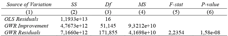
In Table 4, there are GWR improvement component where its SSR is got from the difference between global model and GWR model. In other words, GWR improvement is a reduction due to the use of residual GWR models. By looking at the p-value in column 6 which is the approach of the F distribution with freedom degrees (194.056, 195.087), the null hypothesis can be rejected. In conclusion, with a 95% confidence level, GWR models provide more significant changes in explaining the relationship between the predictor variables and the response variable than OLS models. This means that the predictor variable with varies coefficient geographically able to explain the average per capita household expenditure in DIY better than the constant coefficients across geographic locations.
Table 4. Analysis of varians (ANOVA)
Source of Variation SS Df MS F-stat P-value
(1) (2) (3) (4) (5) (6)
OLS Residuals 1,1933e+13 16
GWR Improvement 4,7673e+12 51,145 9,3212e+10
GWR Residuals 7,1660e+12 171,855 4,1698e+10 2,2354 1,58e-08
3. Determination of Underdeveloped Villages
One objective of this study is to determine the status of a village. If the estimated value of the average per capita household expenditure in a village is under the poverty line, the area is classified as underdeveloped villages. According to BPS, the poverty line of DIY in 2011 was Rp 249.629,00. Based on the established modes from OLS and GWR, from 239 villages Susenas sample, the classification results as follows (Table 5).
Table 5 explains that the consistency of GWR model in classifying the villages is 91,63 percent, higher than the OLS model (89,96 percent). Thus, GWR models are more consistent in classifying the villages than OLS models.
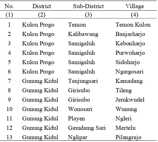
To get the prediction of average per capita household expenditure on nonsampled areas, equation (12) is used. As a result, from 438 villages in DIY there are 13 villages belonging to the underdeveloped villages, presented in Table 6.
Table 5. Consistency of Classification (COC) OLS dan GWR model
Original Data Model Classification
Underdeveloped Non-Underdeveloped Total
COC
(%)
(1) (2) (3) (4) (5) (6)
Underdeveloped 1 6 7
Non-underdeveloped 18 214 232
OLS
Total 19 220 239
89,96
Underdeveloped 5 6 11
Non-underdeveloped 14 214 228
GWR
Total 19 220 239
91,63
Table 6. List of Underdeveloped villages by GWR Model
No. District Sub-District Village
(1) (2) (3) (4)
1 Kulon Progo Temon Temon Kulon 2 Kulon Progo Kalibawang Banjarharjo 3 Kulon Progo Samigaluh Kebonharjo 4 Kulon Progo Samigaluh Purwoharjo 5 Kulon Progo Samigaluh Sidoharjo 6 Kulon Progo Samigaluh Ngargosari 7 Gunung Kidul Tanjungsari Kemadang 8 Gunung Kidul Girisubo Tileng 9 Gunung Kidul Girisubo Jerukwudel 10 Gunung Kidul Wonosari Wunung 11 Gunung Kidul Playen Ngleri 12 Gunung Kidul Gemdamg Sari Mertelu
4. Characteristics of underdeveloped villages
The poor society tends to clustering in certain places, forming proverty clusters in the region (Henniger and Snel, 2002). The exis-tence of this cluster shows similarity or dissimilarity level of poverty in the neigh-boring area. Meanwhile, spatial autocorre-lation can measure the strength of that spatial clustering (Anselin, 1995). Thus, detection of spatial autocorrelation can be used to identify the interaction between the region which causes a higher or lower concentration of poverty level. To see the spatial autocorre-lation in underdeveloped villages in DIY, this study uses Local Indicators of Spatial Association (LISA).
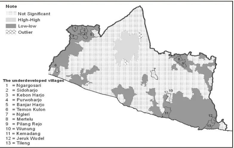
Figure 5 is a map clustering tendency of the average per capita household expenditure estimated by GWR models. The blue, red, and yellow area are significant in a particular
cluster indicating the interaction region. High cluster marked in red are in the city of Yogyakarta and the surrounding villages. It means there is a village which has high ave-rage per capita household expenditure which interacts due to high average per capita house-hold expenditure in the surrounding villages. While the low clusters marked in blue are in the district of Kulonprogo, Bantul, and Gunung Kidul. It means there is a village which has low average per capita household expenditure which interacts due to lower average per capita household expenditure in the surrounding villages.
From Figure 5 it can be seen that there are nine underdeveloped villages in DIY was the low clusters significantly. Meanwhile, four other villages have low average per capita household expenditure, but the interaction was not significant.
Sources: Processing with Software Open GeoDa 10 and ArcGIS 10
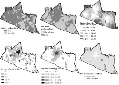
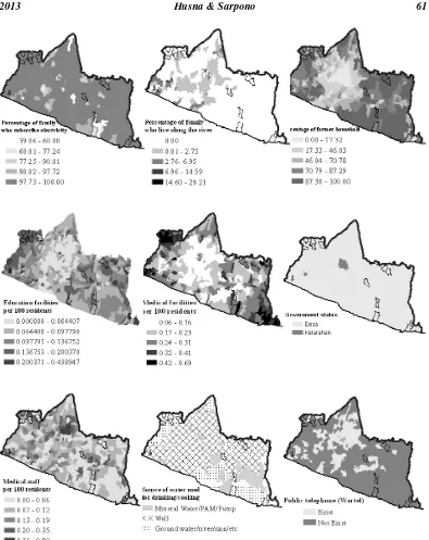
Moreover, we get information about the condition of the 13 underdeveloped villages from Podes. Most of underdeveloped villages are lack in number of population (about 300 people per km square). They are located far from the office of regent, especially in Kulon Progo. Education facilities are good enough. There are a lot of medical facilities consist of Polindes and Posyandu, but they have no hos-pital. They also lack in the number of medical worker. The infrasturctures are not good enough. No one have public telephone and minimarket. About socio-economic factors, most people in underdeveloped villages are farmers. They use firewood to cook. Most of them subscribe electricity but they still depend on ground water, river, or rain to drink or cook. There are malnutrition problems in Ku-lon Progo. More detail information can be seen in Figure 7 (Appendix).
CONCLUSION
GWR models that noted spatial variation are able to explain the relationship between the response variable and the predictor vari-able better than the OLS models. By combin-ing census and survey data, GWR models are very good to small area estimation. In this study GWR model are used to estimate the average per capita household expenditure in the village level. By using the GWR, we get result that there are 13 underdeveloped vil-lages in the Province of Yogyakarta` in 2011, those are: Temon Kulon, Banjarharjo, Kebon-harjo, PurwoKebon-harjo, SidoKebon-harjo, Ngargosari, Kemadang, Tileng, Jerukwudel, Wunung, Ngleri, Mertelu, and Pilangrejo. Some of them are located in Kulonprogo and others are in Gunung Kidul.
Most of underdeveloped villages are lo-cated in Low-Low area. There are interaction between the village which have low expendi-ture and surrounding villages that also have low expenditure. Most of them are lack in number of population, public telecommunica-tion facilities, minimarket, and medical
worker. Most people in underdeveloped vil-lages are farmers. They use firewood to cook. They also get water to drink and cook from ground, river, or rain
IMPLICATIONS
The results show that there are 13 underdeveloped villages in the Province of Yogyakarta in 2011. It can be a reference in determining the pro-poor development prio-rities and deliver direct assistance programs, such as the fuel subsidy.
To improve the welfare of people in un-derdeveloped villages, the government needs to develop the infrastructure in the field of communication. The minimal number of health is also a concern of the government that is expected to improve the health and tackling the problem of malnutrition. In addition, the government needs to encourage the banking sector to be more inclusive and better reach people in remote areas. By the access to capital, we hope that people does not depend on the agricultural sector so that the economy can develop more. PAM is necessary to expand because most of underdeveloped villages are still depend on ground, river, or rain.
government also needs to facilitate inter-re-gional mobility. Secondly, the government needs to reduce the distance by building good infrastructure to reduce transport costs. For example, by increasing the supply of cheap and convenient public transportation. Most of the underdeveloped villages in Kulonprogo located quite far away from the district capital (over 30 km), while Gunung Kidul is moun-tainous geographical location. Whereas, most of society work in the agricultural sector so that they find difficulties to sell the agricul-tural and buy needs that can not be found in the village. Third, the division relates to re-duce inequalities between regions to create inclusive economic development. Another way in which the transition from the rural ar-eas to educate people towards modern society, especially in matters of agriculture and the improvement of the wages system. In addition, managing the social gap can also be done through a fiscal transfer mechanism.
Good communication between the gov-ernment and the people are absolutely neces-sary so that development can be optimized done. The development of underdeveloped villages is expected to push the poverty rate in Yogyakarta.
REFERENCES
Anselin, L., 1988. Spatial Econometrics: Methods and Models. Dordrecht: Kluwer Academic Publishers.
Anselin, L., 1992. Spatial Data Analysis with GIS: An Introduction to Application in the Social Science, Technical Report of Nation Center for Geographic Information and Analysis. Santa Barbara: University of California.
Anselin, L., 1995. Local Indicators for Spatial Association-LISA. Geographical Analy-sis, 27, 93 – 115.
Anselin and Griffith, 1988. Do Spatial Effects Really Matter in Regression Analysis?
Journal of the Regional Science Association, 65, 11-34.
Badan Pusat Statistik, 2004. Penyempurnaan Metodologi Perhitungan Penduduk Mis-kin dan Profil KemisMis-kinan. Jakarta: Badan Pusat Statistik.
Badan Pusat Statistik, 2005. Identifikasi dan Penentuan Desa Tertinggal 2002 Buku I: Sumatera. Jakarta: Badan Pusat Statistik. Badan Pusat Statistik, 2012. Statistik Daerah
Provinsi Daerah Istimewa Yogyakarta 2011. Jakarta: Badan Pusat Statistik Brandon, Vista., 2006. Exploring The Spatial
Patterns and Determinants of Poverty: The Case of Albay and Camarines Sur Provinces in Bicol Region, Philipines, Thesis. Tsukuba: University of Tsukuba. Brunsdon, C., Fotheringham A.S. and
Charlton, M., 1996. Geographically Weighted Regression: A Method for Exploring Spatial Nonstationarity. Geo-graphical Analysis, 28, 281-298.
Brunsdon, C., Fotheringham, A. S. and Charlton, M., 1999. Some Notes on Pa-rametric Significance Tests for Geo-graphically Weighted Regression. Jour-nal of RegioJour-nal Science, 39, 497-524. Brunsdon, C., Fotheringham, A. S. and
Charlton, M., 2002. Geographically Weighted Regression: The Analysis of Spatially Varying Relationships. Chichester: John Wiley and Sons, Ltd. Dimulyo, Sarpono., 2009. Penggunaan
Geo-graphically Weighted Regression-Kriging untuk Klasifikasi Desa Terting-gal [The Using of Geographically Weighted Regression-Kriging for Underdeveloped Villages Classification]. In: Seminar Nasional Aplikasi Teknologi Informasi 2009. Yogyakarta: Universitas Islam Indonesia.
Ginting, Martinus., 1997. Faktor-Faktor yang Berhubungan dengan Status Gizi Balita pada Empat Desa Tertinggal dan Tidak Tertinggal di Kabupaten Pontianak, Pro-pinsi Kalimantan Barat Tahun 1995,
Henninger, N. and Snell, M. 2002. Where Are The Poor? Experiences with the Deve-lopment and Use of Poverty Maps. Washington: World Resources Institute.
Hentschel, J., J.O. Lanjouw, P. Lanjouw, and J. Poggi, 2000. Combining Census and Survey Data to Trace the Spatial Dimension of Poverty: A Case Study of Ecuador. The World Bank Economic Review, 14.
Hurvich C M, Simonoff J S, Tsai C-L, 1998. Smoothing Parameter Selection in Non-parametric Regression Using an Improv-ed Akaike Information Criterion”. Jour-nal of the Royal Statistical Society Series B, 60, 271–293.
Leung, Y., Mei, C. L. and Zhang, W. X., 2000. Statistical Test for Spatial Nonstatio-narity Based on the Geographically Weighted Regression Model. Journal Environment and Planning, 32, 9–32. Rahmawati, R. and Djuraidah, A., 2010.
Regresi Terboboti Geografis dengan Pembobot Kernel Kuadrat Ganda untuk Data Kemiskinan di Kabupaten Jember [Geographical Weighted Regression with Bi-Square Kernel Weighting for Poverty
Data in Jember]. Forum Statistika dan Komputasi, 15 (2).
Sumaryadi, I Nyoman. 1997. Pembangunan Masyarakat Desa dalam Perspektif Pe-nanganan Kemiskinan Melalui Pelaksa-naan Program Inpres Bantuan Pemba-ngunan Desa dan Inpres Desa Tertinggal
[Villagers Development in Poverty Handling through Implementation of Program Inpres Bantuan Pembangunan Desa and Inpres Desa Tertinggal Perspective], Tesis. Jakarta: Universitas Indonesia.
Sukowati, Nisa N. Pola Spasial dan Deter-minan Spasial dari Tingkat Kemiskinan di Nusa Tenggara Barat 2008 [Spatial Pattern and Spatial Determinants of Poverty Level in Nusa Tenggara Barat 2008], Skripsi. Jakarta: Sekolah Tinggi Ilmu Statistik.
World Bank, 2009. World Economic Report 2009: Reshaping Economic Geography. Washington DC: The World Bank. Yrigoyen, C.C. and Rodriguez, I.G., 2008.