Forward-Looking
Christopher A. Swann
A B S T R A C T
In 1996 the Aid to Families with Dependent Children program was replaced with the Temporary Assistance for Needy Families (TANF) program. This paper considers the effects of two specific components of TANF, time limits and work requirements, on employment, marriage, and welfare participa-tion. I use a discrete-choice dynamic programming model and obtain param-eter estimates using data from the Panel Study of Income Dynamics. Policy simulations show that a five-year lifetime time limit results in a 60 percent reduction in welfare use and that a substantial part of this reduction occurs because recipients are forward-looking.
I. Introduction
On August 22, 1996, President Clinton signed legislation that replaced the Aid to Families with Dependent Children (AFDC) program with the Temporary Assistance for Needy Families (TANF) program.1AFDC was introduced in the Social Security Act of 1935 and grew to become the heart of the welfare sys-tem in the United States. It was a means-tested entitlement program that provided cash assistance to single-parent families. Because the size of the cash grant increased with the number of children, decreased with income, and was primarily available for single-parent households, there was a great deal of concern that it created incentives
Christopher A. Swann is a professor of economics at UNC-Greensboro, Greensboro, N.C. This paper has been substantially improved by comments from Todd Stinebrickner and two anonymous referees. The author acknowledges helpful comments on previous versions of this paper from Steven Stern, Michael Brien, Fredrick Holt, Edgar Olsen, and numerous seminar participants. He claims responsibility for all remaining errors. The data used in this article can be obtained beginning October 2005 through September 2008 from Chris Swann, Department of Economics, Box 26165, UNC-Greensboro, Greensboro, N.C. 27412 <chris_swann@uncg.edu>
[Submitted August 2000; accepted October 2003]
ISSN 022-166X E-ISSN 1548-8004 © 2005 by the Board of Regents of the University of Wisconsin System
1. Although the AFDC program has been replaced by the TANF program, I will refer to AFDC frequently in the paper since that was the relevant program over the time period of the data. In addition, except for these first paragraphs, I refer to the AFDC program in the present tense.
for out-of-wedlock childbearing and divorce and disincentives for employment and self-sufficiency.2
The broad Federal guidelines of TANF and the specific policies implemented by the states address a number of concerns raised by critics of the AFDC program. For example, there is an increased emphasis on moving recipients into jobs; states may implement a “family cap” under which benefits do not increase if a recipient has additional children while receiving TANF; and many states have made it easier for two-parent families to receive assistance. While these represent important policy changes in their own right, the centerpiece of the TANF program is a 60-month time limit on Federal cash benefits. As with other aspects of TANF, states have some flexibility regarding time limits and may either implement a shorter time limit or extend the time limit if the additional benefits come from state (rather than Federal) funds.
The shift from a lifetime entitlement to time-limited benefits is a significant change in policy and one with unknown effects. Cross state variation in benefit levels and job training programs has made it possible to learn how these parameters affect welfare participation, but time limits were, outside of some state waiver programs, untested at the time TANF was enacted. The purpose of this paper is to investigate the effect of time limits on welfare participation and other behavior.
In the absence of any behavioral change, it is relatively straightforward to deter-mine how many recipients will be affected by a time limit. In this case, the affected recipients are those who, in the absence of the time limit, accumulate more than 60 months of AFDC receipt over their lifetimes. Duncan, Harris, and Boisjoly (1997) use data from the Panel Study of Income Dynamics (PSID) to construct lifetime measures of AFDC receipt and find that approximately 40 percent of recipients will be affected by the 60-month time limit.
Understanding the consequences of time limits is more difficult once we allow for behavioral effects. If recipients are forward-looking, they may alter their behavior prior to reaching the time limit. For example, in the presence of a time limit, a woman who is deciding whether to participate in AFDC or accept a job offer that makes her ineligible must weigh the potentially higher current period utility derived from receiv-ing AFDC against the fact that she will be spendreceiv-ing some of her eligibility for future AFDC participation. Consequently, the effect of a time limit is likely to be larger if we allow for a behavioral response to the policy change.
A number of studies (for example, Moffitt 1983; Miller and Sanders 1997; Keane and Moffitt 1998; Grogger and Michalopoulos 1999; and Keane and Wolpin 2000) model the decision to participate in AFDC. Of these, Miller and Sanders (1997); Grogger and Michalopoulos (1999); and Keane and Wolpin (2000) allow for forward-looking behavior. Miller and Sanders (1997) focus on human capital accumulation as an explanation for nonparticipation by eligible women rather than on welfare reform. Keane and Wolpin (2000) examine the effect of the parameters of the AFDC program on a number of outcomes for a subset of states, but they do not consider time limits or other TANF-like reforms. Grogger and Michalopoulos (1999) focus specifically on
time limits and other pre-TANF policy changes in Florida. They find that even before any woman has reached the time limit welfare utilization falls by 19 percent. Although the present paper and the paper by Grogger and Michalopoulos (1999) focus on the same question, the econometric strategies are quite different. They test the reduced-form implications of their economic model while this paper estimates the parameters of the economic model directly.
The decision to participate in welfare each period is modeled jointly with the decisions to work or marry using a discrete-choice dynamic programming model where women are assumed to maximize their expected, discounted lifetime utility. Uncertainty exists because future wages, utility, and marriage offers are unknown. The framework is structural in the sense that the empirical analysis is closely tied to the economic problem (potential) recipients are assumed to solve, and, conse-quently, the parameter estimates have a behavioral interpretation. Maximum likeli-hood and data from the Panel Study of Income Dynamics (PSID) are used to estimate the parameters of the econometric model. An advantage of the structural approach is that one may use the parameter estimates to conduct counterfactual pol-icy simulations even though the policies under consideration may not be observed in the data.3
Four different policies are simulated. The first, a 10 percent reduction in the ben-efit reduction rate, provides a comparison point to the previous literature. The other three approximate important aspects of the TANF program. These include a five-year time limit after which benefit end (“benefit termination” time limit); a two-year time limit after which nonexempt recipients must work (“work trigger” time limit); and the combination of the two time limits. Reforms 2 and 3 highlight specific aspects of the TANF program, and the last policy approximates the core structural reforms of TANF.
The reforms are compared across a number of dimensions including their effect on welfare utilization, the choices made by former recipients, their ability to divert ients from welfare altogether, and the degree to which reductions occur because recip-ients “bank” their time for use at a later date. The simulations show that a five-year time limit is associated with a reduction in welfare utilization of about 60 percent. Nineteen percent of this reduction is due to changes in behavior rather than simple “mechanical” reductions.
II. Economic Model and Econometric Specification
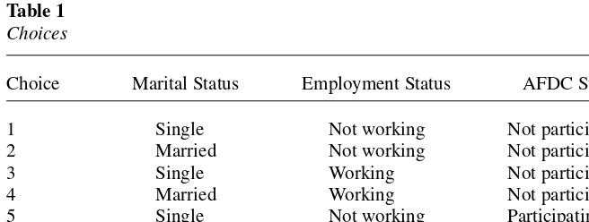
In the economic model each woman makes decisions regarding her marital status, whether she works, and whether she receives AFDC. In a given period she may have as few as two choices or as many as six. The six possible choices are summarized in Table 1. The specific number of choices depends on her particular cir-cumstances in the following ways. She may always choose to be single, not work, and not receive AFDC (Choice 1) or to be single, work, and not receive AFDC (Choice 3).
If she has at least one child younger than 18 years old, she also may choose to be sin-gle, not work, and receive AFDC (Choice 5). If her wage offer is low enough that she is income-eligible, she may choose to be single, work, and receive AFDC (Choice 6). In addition, as discussed below, the model allows for the possibility that marriage is an option in some periods. In the periods when marriage is an option, she may choose to be married, not work, and not receive AFDC (Choice 2) or to be married, work, and not receive AFDC (Choice 4).
The model does not allow married women to receive welfare. Under the AFDC-Unemployed Parent (AFDC-UP) program, married couples are eligible to receive cash assistance, but the AFDC-UP program has stricter eligibility requirements and smaller enrollments than the basic AFDC program. For these reasons, and because it has not been a significant focus of the welfare reform debate, this aspect of AFDC is not modeled.4
A. The Optimization Problem
Each woman is assumed to choose one of the available choices each period in order to maximize her expected, discounted lifetime utility. Let Jtto be the set of choices available at time t. Where necessary, J0,tdenotes the subset of choices when marriage is not an option, and J1,tdenotes the set of choices when marriage is an option. Let dj(t) = 1 if choice jis chosen at time tand dj(t) = 0 otherwise; and let d(t) represent dj(t) stacked over j. The utility maximization problem is
( )t
where Uj(t) is the per-period utility function, βis the discount factor, and Edenotes expectations as of the beginning of the decision-making horizon.
4. AFDC-UP provides benefits to two-parent families where at least one parent has a history of attachment to the labor force and is currently unemployed. In 1985, the regular AFDC program had about 10.9 million recipients compared to only 1.13 million for AFDC-UP (Moffitt 1992). See also Hoynes (1996).
Table 1
Choices
Choice Marital Status Employment Status AFDC Status
1 Single Not working Not participating
2 Married Not working Not participating
3 Single Working Not participating
4 Married Working Not participating
5 Single Not working Participating
B. Specification of Utility
The utility of choice jis assumed to be additive in the pecuniary and nonpecuniary value of the choice:
( )2 Uj( )t =q tj( )+aln(c tj( ))
where qj(t) denotes the nonpecuniary value, cj(t) denotes consumption, and the parameter αweights the effect of consumption relative to leisure.
The nonpecuniary value of the choice captures a number of things including the value of leisure, the disutility of working, and the “stigma” of AFDC participation. Each of these may depend on the woman’s demographic characteristics to reflect, for example, the role of education in the formation of stigma or the role of children in the disutility of work. They may also depend on the woman’s tenure on AFDC, in a marriage, or in an employment spell. For example, stigma may lessen with exposure to the AFDC program; a couple may accumulate marriage-specific capital over the course of their marriage; and preferences for work may evolve through habit formation.
For these reasons, nonpecuniary utility is assumed to depend on the woman’s exogenous characteristics and on tenure variables that evolve endogenously. The spe-cific form of nonpecuniary utility for choice jis
( )3 q tj( )=djXj( )t +wjS tj( -1)+fj( )t
where δjand ςjare vectors of parameters for choice j, Xj(t) is a choice-specific vector of exogenous observed characteristics, Sj(t−1) is a choice-specific vector of endoge-nous “state variables” as of the beginning of period t, and ej(t) is a stochastic shock to the nonpecuniary value of choice jat time t.
The vector Xj(t) includes those variables discussed above that affect the nonpecu-niary value of each choice and are assumed to be exogenous. In the empirical imple-mentation, Xj(t) includes age, education, and indicator equal to one if the woman is black and (for one specification) the number of children younger than 18 years of age. It is assumed that the path of each of these variables is known from the beginning of the decision-making horizon and is not influenced by work, marriage, or welfare participation decisions.
Of these variables, the number of children plays a key role in the model because the presence of children determines eligibility for AFDC, the number of children deter-mines the size of the AFDC benefit, and both the presence and number of children are endogenous to work and marriage decisions. Unfortunately, for reasons to be discussed below, modeling fertility decisions jointly with the other decisions increases the com-putational burden of estimation to such a degree that it is not possible to estimate the parameters of the more general model. Consequently, it is assumed that each woman knows her childbearing profile at the beginning of the problem.5
The state variables Sj(t) include the number of years of lifetime AFDC recipient, the number of years in the current employment spell, and the number of years of the current marriage, but only a subset of these variables is relevant for each of the choices. Specifically, employment tenure is only allowed to affect the utility of con-tinuing to work; AFDC tenure is only allowed to affect utility in the choices involv-ing welfare participation; and marriage tenure is only allowed to affect utility when married. Unlike the elements of Xj(t), these variables evolve endogenously, and their paths are not known at the outset of the optimization problem. The laws of motion for the three tenure variables are given by
( )4 Sa( )t Sa(t 1) d t( ) d ( ),t
5 6
= - + +
( ) ( ) ( ) ( ) ( ) ,
Se t d t d t d t Se t 1 1 and
3 4 6 $
=_ + + i _ - + i
( ) ( ) ( ) ( )
Sm t d t d t Sm t 1 1
2 4 $
=_ + i _ - + i
where t> 1, Sa(t) denotes AFDC tenure at time t, Se(t) denotes employment tenure, and Sm(t) denotes marriage tenure. The initial values for the state variables are all assumed to be zero: Sk(0) = 0 for k= a, e, m.
In the empirical implementation, it is assumed that there is no marginal effect of AFDC tenure after six years and no marginal effect of marriage and employment tenure after four years. This assumption is made in order to reduce the time required to estimate the model and does not imply that, for example, women are limited to only six or fewer years of AFDC receipt.
To this point, the discussion of utility has focused on the nonpecuniary utility of the choices. The other component of utility is consumption. The consumption good is a composite commodity with a price of one. Because there is no saving, consumption in each period is equal to that period’s income and comes directly from the budget constraint.
C. Specification of Income
There are three sources of income in the model. First, a woman receives income when she works. Labor income for women who work and do not receive AFDC is assumed to be 1900 : wwhere wis the hourly wage offer. For women who work and receive AFDC, labor income is assumed to be 500 : w.
Observed wages are used for working women. For women who do not work, the equation governing wage offers is assumed to be
( )5 lnw=cwXw( )t +hw( )t
where Xw(t) is a vector of observed characteristics that includes age, years of educa-tion, an indicator equal to one if the woman is black, an indicator equal to one if the woman resides in the south, the number of years of work experience, and the number of years of lifetime AFDC receipt.
match-ing without introducmatch-ing husband’s characteristics directly into the model. For women who are not married, a potential husband’s hourly wage is given by
( )6 lnwhw=chXhw( )t +hhw( )t
where Xhw(t) is a vector of observed characteristics that includes the woman’s years of education, an indicator equal to one if she is black, an indicator equal to one if she resides in the south, a measure of potential work experience, this measure squared, and the number of years of lifetime AFDC receipt. The measure of potential work experience is the number of years since the woman left school. Under the assumption that men work full-time, full-year, this variable approximates the potential work experience of a male of her cohort.
Once family income is known, one must also consider how it is shared among fam-ily members. An equivalency scale that counts children as one-half adults is used to determine the number of “adult equivalents” in the family (Deaton 1997). The number of adult equivalents (AE) is computed as
( )7 AE=1+0 5. *kidst+1(mt=1)
where kidstis the number of children present at time tand 1(mt= 1) is an indicator function equal to 1 if the woman is married at time tand zero otherwise. The woman’s share of income is computed as ρt= [AE]−1. For example, a single woman with two children receives one-half of family income, and a married woman with these same two children receives one-third.
The final source of income is the AFDC benefit. The AFDC benefit formula is characterized by an income guarantee (G) and a benefit reduction rate (r) that sets the rate at which benefits are reduced as a recipient earns income. Statutorily, the guarantee varies over time, across states, and by family size while the benefit reduc-tion rate only varies over time. However, to account for certain state-specific exemp-tions and deducexemp-tions that I do not consider directly, the empirical implementation uses “effective” guarantees and benefit reduction rates. The effective guarantee varies over time, across states, and by family size while the effective benefit reduc-tion rate varies across states and over time. Under the assumpreduc-tion that working AFDC recipients work 500 hours per year, the annual AFDC benefit for which a fam-ily is eligible is given by
( )8 B X( a( ),t kids w, ) G X( ( ),t kids ) r X( ( ))t 500 w
t = a t - a $ $
where Xa(t) is a vector of year and state of residence, kids
tis the number of children at time t, G(Xa(t), kids
t) is the annual AFDC guarantee, and r(Xa(t)) is the benefit reduction rate. If the wage offer is large enough that the calculated benefit is negative, the family fails the income test and is not eligible for AFDC.
Given these sources of income, the income available for each choice is
( )9 Y t1( )=1,
( ) ,
Y t2 =tt72000$whwA
( ) ,
( ) ,
Under the assumption that there is no saving or dissaving, the per-period budget constraint is
When making her decision, each woman knows whether marriage is an option in the current period, but, depending on her choice, she may be uncertain about whether she will have an offer in the next period. If marriage is an option at time tand she chooses to be married, then marriage is assumed to be an option at time t+1. If, on the other hand, she either does not have a marriage offer at time tor she has an offer and does not accept it, then the probability of receiving a marriage offer at t+1 is Φ(Xm(t+1)
$γm) where Φdenotes the normal distribution function, Xm(t+1) is a vector of individual characteristics (age, education, race, and the number of years of AFDC receipt), and
γmis a vector of unknown characteristics. In general, the probability of a marriage offer at time tdepends on the value of the state variables at time t−1 and the woman’s observed characteristics at time t and is denoted π(S(t −1), Xm(t)).
E. The Dynamic Programming Problem
The form of Equation 12 underscores the sources of uncertainty in the model. When she makes her current period decision, each woman is assumed to know the current period value of each of the stochastic terms, but there is uncertainty over future values of her income, her husband’s income, the stochastic shocks to utility, and, if she chooses to be single this period, the availability of a marriage offer in the next period.
The dynamic programming problem is solved backward recursively. Let Tbe the last period in the decision-making problem. At this point, there is no future, and the individual can form a decision rule for this time period conditional on any value of the state variables. Given this solution, she can solve the problem at time T-1 because she can now compute the expected value of the last period’s best choice given that she knows the parameters of the distributions governing stochastic shocks. Repeating this procedure, it is possible to solve the model for each previous period. This solution is required in order to form the choice probabilities for the likelihood function.6
Estimating this model is computationally challenging because the solution requires knowledge of the value of each choice for each possible combination of the endoge-nous state variables (AFDC tenure, employment tenure, and marriage tenure) at each point in time. This feature of the model makes inclusion of fertility as an endogenous choice extremely difficult. Including fertility as a choice variable doubles the number of choices, but, more importantly, it dramatically increases the size of the state space. For the non-AFDC choices, it may be sufficient to use a state variable such as the number of children ever born (van der Klaauw 1996). Unfortunately, in order to prop-erly account for future AFDC receipt, the entire age distribution of children younger than 18 years old must be considered. Knowing that a woman has two children is not sufficient to capture the value of AFDC because her future eligibility depends on the specific ages of the two children. Making the age distribution of children a state variable is not feasible.
F. The Likelihood Function
The parameters of the model are estimated using the technique of maximum likeli-hood. In order to form the likelihood contributions, distributional assumptions about εj(t), ηw(t), and ηhw(t) must be made. The εj(t)’s are assumed to have an i.i.d. extreme value distribution with mean zero and variance τ2π2/6 where τis a param-eter to be estimated. The ln wage disturbances are assumed to be normally distrib-uted with mean zero and variances of σw2and σhw2 for the women and their husbands, respectively.
Under the extreme value assumption and conditional on particular values for wages, the inner (multidimensional) integral in Equation 12 has a closed form solution:
( ) { ( , ( )) | ( ), ( ) } ( )
whether a marriage offer has been received, and ξ is Euler’s constant. Denoting this closed-form solution by Rm,j(t+1, S(t)) and defining p= p(S(t), Xm(t+1)), the
The closed form solution for the inner integral must be integrated over the distri-butions of the wage disturbances. This integration is accomplished numerically using Gauss-Hermite quadrature with five points (see Judd 1998).
A second consequence of the extreme value assumption is that, conditional on par-ticular values for wages and the presence (m= 1) or not (m= 0) of a marriage offer, the choice probabilities have a closed-form, multinomial logit solution:
t
offer is not observed by the econometrician. For example, wages are not observed for women who do not work, and husband’s wages are not observed for single women. In these cases, the choice probability must be integrated over the appropriate wage distribution(s). This integration is also implemented numerically using five point Gauss-Hermite quadrature.
The likelihood contribution for each of the choices is the probability of the observed choice multiplied by the appropriate wage densities when wages are observed or integrated over the wage densities when wages are not observed. Because the econometrician does not observe whether a marriage offer is received, the likeli-hood contribution also incorporates the probability of receiving a marriage offer. As an example, consider the probability that a woman (single in period t−1) chooses to be single, not work, and receive AFDC in period t. This likelihood contribution is given by
An individual’s likelihood contribution is the product over the years she is in the sample of each year’s contribution, and the sample likelihood is the product of each individual’s contribution. The likelihood function for the full sample is
1 choice specific likelihood contribution. The Berndt, Hall, Hall, and Hausman (1974) technique is used to estimate the standard errors of the parameters.
III. Data
The main data source used in this paper is the Panel Study of Income Dynamics (PSID). The PSID began in 1968 with a sample of 4,802 fami-lies. These families have been interviewed annually since the study began, and the data set contains information on more than 38,000 individuals. One of the advan-tages of the PSID is that the children of sample members are sample members themselves and are followed as they age. A woman enters my sample when she fin-ishes school or establfin-ishes her own household (whichever is earlier), and she leaves the sample either when she leaves the PSID through attrition or in 1992 (the last year of data used in this analysis). Because of the way information is collected in the PSID, all marriage spells are observed. However, a minor child who lives at home and receives AFDC is not asked about her AFDC participation. Because a small percentage of women report receiving AFDC in their first year in the sample (approximately 3 percent), the problem of unobserved receipt is likely to be small, and it is assumed that women do not receive AFDC prior to entering the sample. Additionally, rather than attempting to account for summer employment or after-school jobs, employment prior to entering the sample is disregarded. The justifica-tion for this assumpjustifica-tion is that the types of jobs held while attending school tend to be different than the full-time work envisioned within the model. After select-ing eligible women and rejectselect-ing women who are missselect-ing important information, data are available on 24,563 person-years for 1,530 women for an average of about 16 years per person.
Descriptive statistics for the sample are reported in Table 2. The average woman is about 27 years old, has slightly more than a high school education and 1.26 children. Given that she works (hours > 1000), she works about 1,823 hours per year and earns about $6.85 per hour.8Married women on average have husbands who work about 2,000 hours per year and earn about $10.44 per hour.
A family is assumed to receive AFDC if it reports annual AFDC benefits of at least $100. A woman is assumed to participate in the labor force if she reports at least 1000 hours of work in the year (100 hours if she is also receiving AFDC). The second part of Table 2 describes the percentage of time spent in each state. Women choose to be single, not participate in the labor force, and not participate in the AFDC program about 13 percent of the time. They choose to participate in the AFDC program about 9 percent of the time. Most of the time spent participating in the AFDC program is
spent out of the labor force since women only choose AFDC and employment about 3 percent of the time. The single and working state is chosen 29 percent of the time. Finally, women choose married states almost half of the time.
Beyond simple tabulations of the fraction of time each choice is chosen, it is also helpful to know something about the dynamics of participation. Table 3 shows the number of women who experience different numbers of spells of welfare receipt, mar-riage, and employment. As one would expect, most women do not participate in AFDC. In the sample, 1,167 women out of 1,530 do not participate in AFDC. This compares to 349 women who do not marry during the sample period and only 109 who do not work. The table also shows that a number of women experience multiple spells of AFDC (as well as multiple marriages and multiple employment spells). Just over 41 percent of women who participate in AFDC do so in more than one spell of participa-tion. There is an even higher level of dynamics for employment spells in two senses: more women experience multiple employment spells than experience marriage or wel-fare spells, and these women experience a larger number of transitions (spells).
In addition to the PSID data, information about AFDC benefit levels is required because the model assumes that women know the amount of AFDC they would
Table 2
Descriptive Statistics
Variable Mean Standard Deviation Minimum Maximum
Age 27.37 6.12 16.00 50.00
Education 12.75 1.83 8.00 17.00
Number children < 18 1.26 1.15 0.00 6.00
Black 0.45 0.50 0.00 1.00
Hours of work 1,823.67 481.25 100.00 4,000.00
Hourly wage 6.85 3.77 0.50 34.55
Husband’s hours 2,014.68 822.58 0.00 4,000.00
Husband’s wage 10.44 5.29 0.63 44.46
Choice
Single, not working, 0.132 — — —
no AFDC
Married, not working, 0.206 — — —
no AFDC
Single, working, no 0.298 — — —
AFDC
Married, working, no 0.282 — — —
AFDC
Single, not working, 0.057 — — —
AFDC Single, working,
AFDC 0.028 — — —
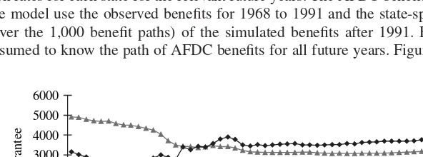
receive if they choose to participate in the program. Given the specification of the AFDC benefit formula, the program is characterized by the guarantee and the benefit reduction rate. For the time period 1967 to the present, one could collect such data for each state for each year. However, the model requires AFDC benefits for future time periods for which data do not exist. In order to project benefits into the future, forecasting equations are estimated.
This estimation uses data collected by Fraker, Moffitt, and Wolf (1985) and McKinnish, Sanders, and Smith (1999). In each of these papers, the researchers used administrative data to estimate “effective” guarantees and benefit reduction rates for the period 1967–91. To forecast benefits, I estimate a separate AR(1) model in first dif-ferences for the guarantee for one adult and one child, for a second child, for a third (or higher order) child, and for the benefit reduction rate for each state. The parame-ters from this estimation are used to simulate 1,000 paths of benefits and benefit reduc-tion rates for each state for the relevant future years. The AFDC benefit calculareduc-tions in the model use the observed benefits for 1968 to 1991 and the state-specific averages (over the 1,000 benefit paths) of the simulated benefits after 1991. Each woman is assumed to know the path of AFDC benefits for all future years. Figure 1 depicts the
Table 3
Count of People by Number of Spells
Number of Spells AFDC Marriage Employment
0 1,167 349 109
1 213 918 624
2 100 216 446
3 46 42 245
4 4 3 67
5 2 2 17
6 0 0 3
7 0 0 0
0 1000 2000 3000 4000 5000 6000
1967 1972 1977 1982 1987 1992 1997 2002 2007 2012 Year
Guarantee
0 0.1 0.2 0.3 0.4 0.5
Benef
it Reduction Rate
Guarantee for a Family of Two Benefit Reduction Rate
Figure 1
annual average (over states) benefit for a family of two (one adult and one child) and the benefit reduction rate over the time period from 1967 to 2015. The figure shows the fall in real benefits during the 1970s and 1980s. The benefit reduction rate is increas-ing durincreas-ing the 1970s and 1980s and is almost constant at about 0.30. Although not shown, benefits are computed for a second child and a third (or higher birth order) child. Given information on the number of children, the state of residence, the year, and the wage offer, these parameters are used to compute the family’s AFDC grant.
IV. Results
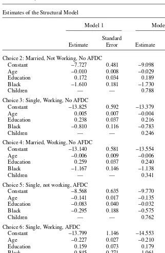
Table 4 presents the estimation results for two different models.9The two specifications help provide some understanding of the role children play in these decisions. In “Model 2,” the utility of each choice depends on age, education, race, and the number of children younger than 18 years old. “Model 1” omits the number of children from the nonpecuniary utility function. However, in all cases the num-ber of children is assumed to be known and determines eligibility for AFDC, the level of benefits, and the share of family income. For each specification, the utility function parameters are found in Panel A and other parameters are found in Panel B.
The first five rows of Panel A in Table 4 are the estimates the parameters associated with the nonpecuniary utility of being married and working, the second five rows are the estimates of the nonpecuniary utility of being single and working and so on. The table entries measure the marginal impact of the observed characteristic on the utility in the state under consideration relative to the base state (single, not working, no AFDC). For example, the fact that the coefficient on “children” for choice 2 in Model 2 is 0.788 means that having an additional child while married and not work-ing increases utility by 0.788 relative to the base state of swork-ingle, not workwork-ing and not participating in AFDC. Because income (consumption) is assumed to enter the model in log form and the coefficient on log income is fixed at one, the coefficients are in terms of log income.
Several conclusions can be drawn from Table 4. First, the estimates imply that women are forward-looking (see Panel B). The specific point estimate of the discount factor depends on the model specification with estimates ranging from 0.81 to 0.84. These estimates are similar to Keane and Wolpin’s (1997) estimate of 0.78 for a model of career choice by young men. They are important because, as discussed in the introduction, the degree to which women are forward-looking affects the size (and existence) of the behavioral response to the policy change: If recipients are not forward-looking, there will be no behavioral response to a time limit.
The estimates in Panel A of Table 4 show a number of consistent results: (1) blacks receive significantly less utility in the married choices than whites; (2) education is positively associated with each choice except for receiving AFDC while not working; and (3) for the model that includes the number of children in the utility function, the nonpecuniary utility of children is highest for married women who do not work and
Table 4
Panel A: Utility Function Parameters
Estimates of the Structural Model
Model 1 Model 2
Standard Standard
Estimate Error Estimate Error
Choice 2: Married, Not Working, No AFDC
Constant −7.727 0.481 −9.098 0.448
Age −0.010 0.008 −0.029 0.008
Education 0.172 0.034 0.189 0.034
Black −1.610 0.181 −1.730 0.188
Children — — 0.788 0.062
Choice 3: Single, Working, No AFDC
Constant −13.825 0.592 −13.379 0.585
Age 0.005 0.007 −0.004 0.006
Education 0.238 0.037 0.216 0.035
Black −0.810 0.116 −0.783 0.108
Children — — 0.246 0.040
Choice 4: Married, Working, No AFDC
Constant −13.140 0.581 −13.554 0.596
Age −0.006 0.009 −0.006 0.007
Education 0.259 0.037 0.240 0.036
Black −1.167 0.146 −1.138 0.138
Children — — 0.341 0.041
Choice 5: Single, not working, AFDC
Constant −8.568 0.635 −9.770 0.612
Age −0.141 0.017 −0.135 0.017
Education −0.083 0.040 −0.032 0.037
Black −0.295 0.188 −0.575 0.184
Children — — 0.762 0.073
Choice 6: Single, Working, AFDC
Constant −13.799 1.146 −14.553 1.099
Age −0.227 0.027 −0.210 0.027
Education 0.159 0.073 0.179 0.068
Black −0.845 0.271 −1.061 0.257
Children — — 0.763 0.103
State Variables
AFDC tenure 1.724 0.143 1.470 0.134
Marriage tenure 0.233 0.059 0.260 0.055
for single women who receive AFDC. This last result occurs in spite of the fact that the effect of family size on benefits is incorporated in the model and may occur because the value of AFDC used in the paper includes only the cash benefit and excludes the value of food stamps and Medicaid.
Table 4
Panel B: Wages Equations and Other Parameters
Estimates of the Structural Model
Model 1 Model 2
Standard Standard
Estimate Error Estimate Error
Own wage equation
Constant 0.103 0.015 −0.291 0.121
Age 0.005 0.0004 0.005 0.0004
Education 0.103 0.001 0.108 0.084
Black −0.067 0.004 −0.067 0.004
South −0.153 0.004 −0.153 0.004
Work tenure 0.119 0.002 0.120 0.002
AFDC tenure −0.065 0.002 −0.067 0.002
Variance 0.469 0.001 0.469 0.001
Husband’s wage equation
Constant 1.444 0.015 1.442 0.015
Education 0.048 0.001 0.048 0.001
Black −0.186 0.005 −0.187 0.005
South −0.112 0.004 −0.111 0.004
Work tenure 0.033 0.002 0.033 0.002
Work tenure squared −0.072 0.007 −0.070 0.007
AFDC tenure −0.048 0.002 −0.048 0.003
Variance 0.486 0.001 0.486 0.001
Marriage probability
Constant −0.383 0.116 −0.291 0.121
Age −0.026 0.003 −0.027 0.003
Education 0.014 0.008 0.011 0.008
Black −0.463 0.030 −0.465 0.030
AFDC tenure −0.007 0.016 −0.013 0.016
Other variables
β 0.814 0.014 0.835 0.013
τ 2.786 0.208 2.560 0.207
The coefficients on the tenure variables are all positive and statistically significant. For AFDC, this effect ranges in magnitude from 1.47 to 1.72. The consequence of this positive effect is that, holding all else constant, women become increasingly unlikely to leave AFDC as they accumulate tenure on the program. There are a number of dif-ferent interpretations of this duration effect. It may represent a woman’s changing cir-cumstances as she learns the rules of the welfare system, or it may serve as a proxy for changing preferences if the stigma of receiving cash assistance diminishes with exposure to the program. There are similar though smaller effects for marriage and employment duration.
It is well known, however, that duration dependence may also be the result of uncon-trolled unobserved heterogeneity (for example, Heckman and Singer 1984; Blank 1989). Because the model does not control for unobserved differences across women, it is not possible to separate these two effects. If the model were extended to allow for unobserved preferences for work, welfare, and marriage, one would expect that some of the persistence in choices across a person’s lifetime that is now attributed to duration would be attributed to these unobserved preferences. Consequently, the observed dura-tion effect would be smaller if unobserved differences were allowed and significant.
The wage equation parameters are quite consistent across the two specifications. Education and work experience each increase wages, and being black and/or living in the south reduces wages. The coefficients in the husband’s wage equation show the effect of the woman’s characteristics on her (potential) husband’s wages. Again edu-cation and experience have positive effects on wages (though experience is qua-dratic), while being black lowers wages. Lifetime AFDC tenure reduces both own and husband’s wages in each model.
Finally, the marriage offer parameters show that race is the most significant factor in determining the probability of a marriage offer. For example, the model predicts that a 20 year old white woman with a high school education and no past AFDC receipt has a 23 percent chance of receiving a marriage offer while a black woman with the same characteristics has an 11.4 percent chance. If this same black woman has five years of AFDC receipt, the probability falls to 10.7 percent.
V. Model Fit
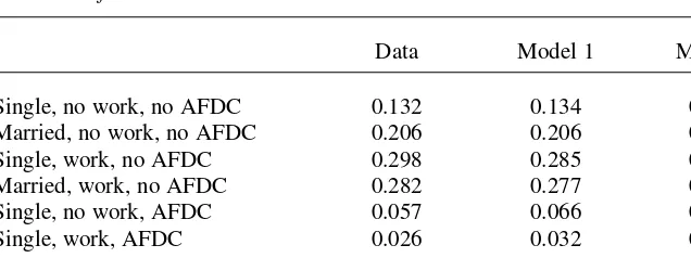
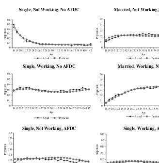
Although the likelihood values in Table 4 provide information about how well each model performs relative to the other, they do not provide any informa-tion about how well either of the models fits the data. To test within-sample fit, 1,000 sequences of welfare, work, and marriage choices are predicted for each woman, and these predicted choices are compared to the actual choices. Table 5 presents the sample proportions from the data and for each model.
such as this one to fail goodness-of-fit tests (for example, Berkovec and Stern 1991; Keane and Wolpin 1997; Brien, Lilliard, and Stern 2001).
Even if the model had exactly predicted the aggregate proportions, it is possible that the model could predict choices across the lifecycle very poorly. The six panels of Figure 2 explore this issue. These figures compare observed and predicted propor-tions (for Model 1) from age 18 to 42. With the exception of Choice 2 (married, not working, and no AFDC), the model captures the general shape of the lifecycle pro-files well. For this choice, the model fits the overall proportion well, but underpredicts this choice during the early 30s and overpredicts it in the teens and late 30s.
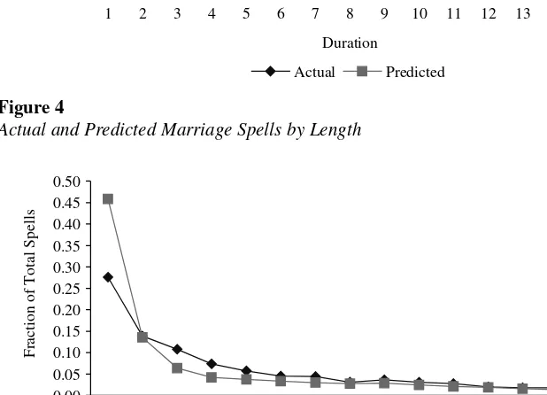
These figures still focus on aggregate proportions rather than on individual spells. Figures 3 through 5 present information about how well the model predicts spell lengths. Figure 3 shows that about 40 percent of all AFDC spells in the PSID sample last one year while about 58 percent of AFDC spells in the simulation last one year. It also shows that the model slightly underpredicts the number of spells longer than three years. Consequently the model is overpredicting transitions on and off the AFDC program. The results for employment spells are similar, but the model does a much better job of fitting the distribution of spell lengths for marriage. Some of this difference may be the result of the uncertainty over future marriage offers that dis-courage women who generally prefer marriage from divorcing in the face of a bad draw of the current-period disturbances.
VI. Policy Simulations
A. MethodologyThe methodology for the simulations is very simple. First, using the same AFDC rules used to estimate the model, a baseline set of simulated choices is obtained. To imple-ment a reform, some aspect of welfare policy is changed, and the process is repeated. Each reform holds everything constant except the policy under consideration, and any change in behavior is attributed to the change in policy. The results of the simulations
Table 5
Goodness of Fit
Data Model 1 Model 2
Single, no work, no AFDC 0.132 0.134 0.136
Married, no work, no AFDC 0.206 0.206 0.191
Single, work, no AFDC 0.298 0.285 0.294
Married, work, no AFDC 0.282 0.277 0.281
Single, no work, AFDC 0.057 0.066 0.066
Single, work, AFDC 0.026 0.032 0.032
χ2-Statistic 75.29 91.02
Single, Not Working, No AFDC
Married, Not Working, No AFDC
0
Observed and Predicted Choices Over the Lifecycle—Model 1
0.00
are found in Table 6. The simulations are conducted for both Model 1 and Model 2, but the table includes results for only Model 1. This specification is chosen because it fits the data better than Model 2, because of a desire to minimize the effect of children in the model, and because the two sets of simulations are similar.
B. Decrease in the Benefit Reduction Rate
Although not part of TANF, one way to encourage welfare recipients to work is to increase the reward for working. Because welfare benefits are reduced as earned income increases, the net wage rate increases as the benefit reduction rate falls. A potential
down-0.00
1 2 3 4 5 6 7 8 9 10 11 12 13 14 15 0.02
0.04 0.06 0.08 0.10 0.12 0.14
Duration
Fraction of Total Spells
Actual Predicted
Figure 4
Actual and Predicted Marriage Spells by Length
0.00 0.05 0.10 0.15 0.20 0.25 0.30 0.35 0.40 0.45 0.50
1 2 3 4 5 6 7 8 9 10 11 12 13 14 15
Fraction of Total Spells
Actual Predicted Duration
Figure 5
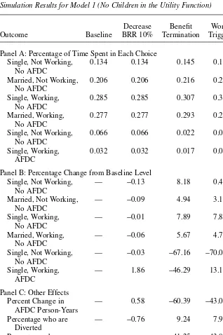
Table 6
Simulation Results for Model 1 (No Children in the Utility Function)
Decrease Benefit Work TANF
Outcome Baseline BRR 10% Termination Trigger Core
Panel A: Percentage of Time Spent in Each Choice
Single, Not Working, 0.134 0.134 0.145 0.135 0.142
No AFDC
Married, Not Working, 0.206 0.206 0.216 0.213 0.217 No AFDC
Single, Working, 0.285 0.285 0.307 0.307 0.313
No AFDC
Married, Working, 0.277 0.277 0.293 0.290 0.296
No AFDC
Single, Not Working, 0.066 0.066 0.022 0.020 0.015
No AFDC
Single, Working, 0.032 0.032 0.017 0.036 0.017
AFDC
Panel B: Percentage Change from Baseline Level
Single, Not Working, — −0.13 8.18 0.43 5.82
No AFDC
Married, Not Working, — −0.09 4.94 3.10 5.27
No AFDC
Single, Working, — −0.01 7.89 7.80 9.92
No AFDC
Married, Working, — −0.06 5.67 4.74 6.87
No AFDC
Single, Not Working, — −0.03 −67.16 −70.02 −77.66 No AFDC
Single, Working, — 1.86 −46.29 13.15 −45.17
AFDC
Panel C: Other Effects
Percent Change in — 0.58 −60.39 −43.04 −67.12
AFDC Person-Years
Percentage who are — −0.76 9.24 7.97 12.00
Diverted
Percentage who — — 41.25 43.06 47.14
make Behavioral Change
Behavioral Change — — 31.45 13.90 21.63
as Percentage of Reduction
side of this policy is that the decrease in the benefit reduction rate increases break-even income and thus the number of women who are income-eligible (and who participate).
The results in Table 6 show that a 10 percent reduction in the benefit reduction rate results in very small reductions in the amount of time spent in each of the choices except for combining work and welfare which increases by about 1.86 percent. The small size of the effect is consistent with previous work including Moffitt (1983) who found that decreasing the benefit reduction rate by 0.10 increased participation probabilities by 1.69 percent and Keane (1995) who found that reducing the benefit reduction rate by 50 percent increased participation probabilities by 2.8 percent.
C. Five-year Time Limit
While many authors have studied changes in the benefit reduction rate, time limits have not been widely studied. This omission is important because the 60-month life-time limit on benefits is arguably the most significant component of the TANF pro-gram. The concept of a time-limit may seem straightforward, but Moffitt and Pavetti (1999) point out that states have implemented a number of different types of limits. In some cases, reaching the time limit triggers a requirement to work while in others reaching the limit results in the termination of benefits. The next reform considered, a five-year benefit termination time limit, approximates TANF’s 60-month time limit on Federal benefits.
Imposing a time limit on welfare receipt leads to a dramatic reduction in welfare utilization. Table 6 shows that the time spent receiving welfare while not working falls from 6.6 percent to 2.2 percent—a drop of about 67 percent from the baseline level. The reduction in the time spent combining work and welfare, about 46 percent, is smaller though still substantial. Combining the two categories, the overall reduction in time spent on welfare is about 60 percent.
The model makes predictions about the choices made by the women who leave AFDC, and time spent in each of the non-AFDC choices increases. The largest effect, an 8.18 percent increase, is in the time spent being single and not working. In the context of this model, that choice can be thought of as living with friends or family or working part-time. There is a slightly smaller increase in the time spent being single and working and smaller still increases in marriage.10The relatively
small increases in marriage are, at least in part, a result of the uncertainty about marriage offers.
This simulation predicts that about 9 percent of baseline recipients will be diverted from the program if a time limit is implemented. The fact that recipients are diverted from the program highlights the distinction between a time limit’s “mechan-ical” effect as opposed to its “behavioral” effect (Ashenfelter 1983). The mechanical effect is the reduction that occurs because anyone who previously participated for more than five years must cut back to five or fewer years. If women are myopic, this is the only effect a time limit will have. However, if women are forward-looking, there is a second effect where women who participated for more years than the time
limit in the baseline cut back to fewer years than the time limit or where women who do not reach the time limit in the baseline simulation nonetheless reduce their utilization. This phenomenon is frequently referred to as “banking” or “hoarding” time (Moffitt and Pavetti 1999).
More than 40 percent of baseline recipients respond behaviorally in the sense that they reduce their usage in some way beyond a pure mechanical effect. The reduction in person-years due to the behavioral effect is about 31 percent of the total reduction or about 19 percent of baseline AFDC. This result is remarkably similar to Grogger and Michalopoulos’ (1999) estimate of a 19 percent reduction even before the time limit takes effect, and it implies that a substantial proportion of the reduction in wel-fare utilization is due to a behavioral response that is missed by models that due not allow for forward-looking behavior.
Because the behavioral effect is 19 percent of baseline, the mechanical reduction is 41 percent (since the overall reduction is about 60 percent). This result is quite simi-lar to Duncan, Harris, and Boisjoly’s (1999) conclusion that 40 percent of recipients would be affected by a time limit—in spite of the fact that they measure the fraction of recipients who will be affected rather than the reduction in person-years. In fact, although it is not discussed above, the baseline simulation predicts that 37.4 percent of recipients will accumulate five years of lifetime AFDC in the absence of a time limit.
D. Work Trigger Time Limit
Under TANF, recipients must work or engage in work activities after receiving benefits for 24 months. Single women with children younger than six years old who cannot find childcare are exempt from the work requirement, and states may exempt other groups such as women with children younger than one year old. To approximate the TANF pol-icy, the next reform imposes of a work trigger time limit after two years of receipt with the provision that women with children younger than three years old are exempt.
This policy results in a large (70 percent) decrease in the time spent not working and receiving AFDC. Unlike the benefit termination time limit, there is an increase in the time spent combining work and welfare. The overall effect is a 43 percent reduc-tion in time spent receiving welfare. Perhaps because of the addireduc-tional work experi-ence while on welfare, this reform has a comparatively large effect on the amount of time women spend working—particularly for women who remain single.11
Like the limit on lifetime benefits, this reform has both mechanical and behavioral effects. In the case of the work requirement, nonexempt women who have received AFDC for two years are no longer allowed to receive AFDC without working. Thus, any reduction for women in this circumstance is mechanical. Because the value of AFDC is lower due to these restrictions, eligible women may also choose not to par-ticipate.12 About 43 percent of recipients respond to the work requirement with a
11. If unobserved heterogeneity were added to the model, we would expect the simulations to have a smaller effect because some recipients would have a strong “taste” for AFDC and would be less likely to leave even in the presence of an impending time limit.
behavioral reduction that accounts for almost 14 percent of the overall reduction in utilization.
E. “TANF Core”
Individually, the two time limits have somewhat different effects on choices. The final simulation combines the five-year benefit termination time limit with the two-year work trigger time limit to approximate the core of the TANF reforms.
The effect of this reform on participation most closely mirrors, and is somewhat larger than, the benefit termination time limit by itself. The time spent receiving AFDC without working falls by 5.1 percentage points (almost 80 percent), and the time spent combining work and welfare falls by more than 45 percent. The pattern of choices made by former recipients is similar to those made in the case of the time limit above though the largest effect is on the decision to work.
Given that the two policies together have a larger effect on choices than either pol-icy by itself, it is not surprising that the combined polpol-icy also has a larger effect on most of the behavioral measures. Twelve percent of baseline recipients are diverted from the program, and almost 50 percent of recipients make a behavioral change that accounts for 21 percent of the reduction in AFDC. These results imply that 14.5 per-cent of the 67.12 perper-cent reduction in AFDC use is behavioral and the remaining 52.6 percent (= 67.12 −14.5) is mechanical.
VII. Conclusion
The goal of this paper has been to understand the effect of time limits on welfare participation and other behavior when women are forward-looking. Toward this end, I employ a discrete-choice dynamic programming framework and estimate the parameters of the structural model using maximum likelihood and data from the PSID.
Policy simulations for the preferred specification of utility show that a five-year benefit termination time limit leads to a 9 percent reduction in recipients and a 60 per-cent reduction in person-years of AFDC receipt. Almost one-third of this reduction is behavioral and is missed by models that do not account for forward-looking behavior. A two-year work trigger time limit results in a smaller—though still significant— overall reduction in time on AFDC with an increase in the amount of time spent com-bining work and welfare. When the two time limits are combined to approximate the core of the TANF program, the effect is dominated by the benefit termination time limit. The reductions are larger than either time limit separately, and the general pattern of choices mirrors the benefit termination time limit.
Second, the estimation results show significant duration effects for welfare, marriage, and work. If the model were extended to allow for unobserved heterogeneity, these duration effects would likely be smaller, and consequently the effects of welfare reform would be smaller because women with a relative distaste for work and mar-riage would be less likely to leave AFDC even when a time limit is implemented. In spite of the limitations, however, the model provides a framework to better understand how time limits affect the decisions made by welfare recipients.
References
Ashenfelter, Orley. 1983. “Determining Participation in Income-Tested Social Programs.”
Journal of the American Statistical Association78(383):517–25.
Bane, Mary Jo, and David Ellwood. 1994. Welfare Realities: From Rhetoric to Reform
Cambridge, Mass.: Harvard University Press.
Berkovec, James, and Steven Stern. 1991. “Job Exit Behavior of Older Men.” Econometrica. 59(1):189–210.
Berndt, Ernst, Bronwyn Hall, Robert Hall, and Jerry Hausman. 1974. “Estimation and Inference in Nonlinear Statistical Models.” Annals of Economic and Social Measurement
3:653–65.
Blank, Rebecca. 1989. “Analyzing the Length of Welfare Spells.” Journal of Public Economics39(3):245–73.
Brien, Michael, Lee Lilliard, and Steven Stern. 2001. “Cohabitation, Marriage, and Divorce in a Model of Match Quality.” Unpublished.
Deaton, Angus. 1997. The Analysis of Household Surveys: A Microeconomic Approach to Development Policy. Baltimore: The Johns Hopkins University Press.
Duncan, Greg, Kathleen Mullan Harris, and Johanne Boisjoly. 1997. “Time Limits and Welfare Reform: New Estimates of the Number and Characteristics of Affected Families.” Unpublished.
Fraker, Thomas, Robert Moffitt, and Douglas Wolf. 1985. “Effective Tax Rates and Guarantees in the AFDC Program, 1967–1982.” Journal of Human Resources
20(2):251–63.
Grogger, Jeffrey, and Charles Michalopoulos. 1999. “Welfare Dynamics under Time Limits.” Unpublished.
Heckman, James and Burton Singer. 1984. “A Method for Minimizing the Impact of Distributional Assumptions in Econometric Models for Duration Data.” Econometrica
52(2):271–320.
Hoynes, Hilary. 1996. “Welfare Transfers in Two-Parent Families: Labor Supply and Welfare Participation under AFDC-UP.” Econometrica64(2):295–332.
Judd, Kenneth. 1998. Numerical Methods in Economics. Cambridge, Mass.: The MIT Press. Keane, Michael. 1995. “A New Idea for Welfare Reform.” Federal Reserve Bank of
Minneapolis Quarterly Review19(2):2–28.
Keane, Michael, and Robert Moffitt. 1998. “A Structural Model of Multiple Welfare Program Participation and Labor Supply.” International Economic Review39(3):553–89.
Keane, Michael, and Kenneth Wolpin. 1997. “The Career Decisions of Young Men.” Journal of Political Economy105(3):473–522.
———. 2000. “Estimating Welfare Effects Consistent with Forward-Looking Behavior, Part II: Empirical Results.” Unpublished.
McKinnish, Terra, Seth Sanders, and Jeff Smith. 1999. “Estimates of Effective Guarantees and Tax Rates in the AFDC Program for the Post-OBRA Period.” Journal of Human Resources
34(2):312–45.
Miller, Robert, and Seth Sanders. 1997. “Human Capital Development and Welfare Participation.” Carnegie-Rochester Conference Series on Public Policy46(0):1–43. Moffitt, Robert. 1983. “An Economic Model of Welfare Stigma.” American Economic Review
73(5):1023–35.
———. 1992. “Incentive Effects of the U.S. Welfare System: A Review.” Journal of Economic Literature30(1):1–61.
Moffitt, Robert, and LaDonna Pavetti. 1999. “Time Limits.” Unpublished.
Rust, John. 1987. “Optimal Replacement of GMC Bus Engines: An Empirical Model of Harold Zurcher.” Econometrica55(5):999–1033.