Full Terms & Conditions of access and use can be found at
http://www.tandfonline.com/action/journalInformation?journalCode=ubes20
Download by: [Universitas Maritim Raja Ali Haji] Date: 12 January 2016, At: 22:51
Journal of Business & Economic Statistics
ISSN: 0735-0015 (Print) 1537-2707 (Online) Journal homepage: http://www.tandfonline.com/loi/ubes20
Macroeconomic Forecasting With
Mixed-Frequency Data
Michael P Clements & Ana Beatriz Galvão
To cite this article: Michael P Clements & Ana Beatriz Galvão (2008) Macroeconomic Forecasting With Mixed-Frequency Data, Journal of Business & Economic Statistics, 26:4, 546-554, DOI: 10.1198/073500108000000015
To link to this article: http://dx.doi.org/10.1198/073500108000000015
Published online: 01 Jan 2012.
Submit your article to this journal
Article views: 399
View related articles
Macroeconomic Forecasting With
Mixed-Frequency Data: Forecasting
Output Growth in the United States
Michael P. C
LEMENTSDepartment of Economics, University of Warwick, Coventry, CV4 7AL, U.K. (M.P.Clements@warwick.ac.uk)
Ana Beatriz G
ALVÃOQueen Mary, University of London, London, E1 4NS, U.K. (a.ferreira@qmul.ac.uk)
Many macroeconomic series, such as U.S. real output growth, are sampled quarterly, although potentially useful predictors are often observed at a higher frequency. We look at whether a mixed data-frequency sampling (MIDAS) approach can improve forecasts of output growth. The MIDAS specification used in the comparison uses a novel way of including an autoregressive term. We find that the use of monthly data on the current quarter leads to significant improvement in forecasting current and next quarter output growth, and that MIDAS is an effective way to exploit monthly data compared with alternative methods.
KEY WORDS: Forecasting; Mixed-frequency data; U.S. output growth.
1. INTRODUCTION
The unavailability of key macroeconomic variables, such as GDP (or GNP), at frequencies higher than quarterly has led to the specification of many macroeconometric models on quar-terly data. We consider the usefulness of information available at higher frequencies, such as monthly data, for forecasting out-put growth. A range of leading and coincident indicator vari-ables at a monthly frequency are available. If all of the varivari-ables in the model must to be sampled at the same frequency, then data available at the monthly frequency must be converted to the quarterly frequency by, for example, averaging the months (or taking the last month in the quarter), and information on the first month (or first two months) of the quarter being forecast is discarded.
In this article we explore whether the mixed data sam-pling (MIDAS) approach of Ghysels, Santa-Clara, and Valka-nov (2004) and Ghysels, Sinko, and ValkaValka-nov (2006b) can be successfully adapted to the modeling and forecasting of a key U.S. macroeconomic variable: U.S. output growth. MIDAS al-lows sampling of the regressand and regressors at different frequencies. Typically, the regressand is sampled at the lower frequency. With few exceptions, MIDAS has been used for high-frequency financial data (see, e.g., Ghysels et al. 2006a), although Ghysels and Wright (2006) looked at survey-based macroeconomic forecasts. We compare the results of using MIDAS to forecast output growth with two other approaches that exploit monthly data. The first of these approaches is an extension to the models used by Koenig, Dolmas, and Piger (2003), and the second is a two-step procedure that generates forecasts of missing monthly indicator values, which are then averaged to generate quarterly observations. The MIDAS spec-ification used in the comparison uses a novel way of including an autoregressive (AR) term.
Looking ahead to the results, we find that the use of within-quarter information on monthly indicators can result in marked reductions in RMSE compared with quarterly-frequency AR or AR distributed-lag (ADL) models. Within the set of models that use monthly information, MIDAS fares well across the set of in-dicators that we consider. Coupled with their flexibility and ease
of use, MIDAS models provide an attractive way of exploiting the information in monthly indicators.
These findings are based on a recursive out-of-sample fore-casting exercise that uses “conventional” real-time data. As ex-plained by Koenig et al. (2003), the use of real-time data is clearly preferable to the use of final-revised data for estima-tion and evaluaestima-tion purposes, because out-of-sample forecast-ing exercises based on final-revised data may exaggerate the predictive power of explanatory variables relative to what actu-ally could have been achieved at the time (Diebold and Rude-busch 1991; Orphanides 2001; Orphanides and van Norden 2005; Faust, Rogers, and Wright 2003). Koenig et al. (2003) noted that the way in which real-time data are conventionally used in forecast comparison exercises is based on the use of end-of-sample vintage data. They argued that this approach to real-time estimation and forecasting may be suboptimal, that “at every date within a sample, right-side variables ought to be the most up-to-date estimates availableat that time” (Koenig et al. 2003, p. 618, described as strategy 1 on p. 619). We find that Koenig et al.’s suggestion to use real-time vintage data to esti-mate forecasting models improves forecast accuracy, and that our main conclusions are unchanged: The inclusion of monthly data in the forecasting problem can dramatically reduce RMSE, and MIDAS is an effective way of incorporating monthly data.
The rest of the article is organized follows. Section 2 briefly reviews the MIDAS approach of Ghysels et al. (2004, 2006b) and proposes an extension that facilitates the application of MIDAS to macroeconomic data, namely the inclusion of an AR component. It also describes the two other approaches to using monthly indicator data to generate forecasts of quarterly output growth. Section 3 contains the out-of-sample forecast comparison exercise, split into five parts. Section 3.1 describes our use of monthly and quarterly vintages to estimate and cast in real time. Section 3.2 compares the MIDAS–AR fore-casts against the quarterly AR model forefore-casts using both a
© 2008 American Statistical Association Journal of Business & Economic Statistics October 2008, Vol. 26, No. 4 DOI 10.1198/073500108000000015
546
Clements and Galvão: Macroeconomic Forecasting With Mixed-Frequency Data 547
conventional real-time vintage data approach and final-revised data, to see whether the incorporation of monthly indicator data in the forecasting model results in significant improvements in forecast accuracy. Section 3.3 compares alternative ways of in-corporating monthly data into the forecasting problem. Sec-tion 3.4 investigates the use of real-time vintage data in the forecast comparison exercise. Finally, Section 3.5 compares the multiple-indicator model forecasts with combining individual model forecasts. Section 4 offers some concluding remarks.
2. THE MIDAS REGRESSION APPROACH
The MIDAS models of Ghysels et al. (2004, 2006b) are closely related to distributed lag models (see, e.g., Dhrymes 1971; Sims 1974). The response of the dependent variable to the higher-frequency explanatory variables is modeled using highly parsimonious distributed lag polynomials, as a way of preventing the proliferation of parameters that might otherwise result and of side-stepping difficult issues related to lag-order selection. Parameter proliferation could be especially impor-tant in financial applications, where, say, daily volatility is re-lated to 5-minute interval intraday data (so that a day’s worth of observations amounts to 288 data points), but parsimony also is likely to be important in typical macroeconomic applica-tions, where quarterly data are related to monthly data, given the much smaller numbers of observations typically available. Modeling the coefficients on the lagged explanatory variables as a distributed lag function allows for long lags, with the need to estimate only a small number of parameters.
The basic MIDAS model for a single explanatory variable, andh-step-ahead forecasting, is given by
yt=β0+β1B ters), m is the higher sampling frequency (m=3 when x is monthly andyis quarterly), and, as shown,L1/moperates at the higher frequency. All of the parameters of the MIDAS model depend on the horizonh(although this is suppressed in the no-tation), and forecasts are computed directly without the need for forecasts of explanatory variables. An “exponential Almon lag” function (Ghysels et al. 2004, 2006b) parameterizesb(k;θ)as
b(k;θ)= exp(θ1k+θ2k 2)
K
k=1exp(θ1k+θ2k2)
. (2)
Because macroeconomic forecasts often are produced a number of times during each quarter, monthly data on relevant indica-tors for the quarter being forecast sometimes will be available. For example, the staff of the Board of Governors of the Fed-eral Reserve prepare forecasts sevFed-eral times each quarter for the meetings of the Open Market Committee (see Karamouzis and Lombra 1989; Joutz and Stekler 2000). For illustrative pur-poses, suppose that the value ofxin the first month of the quar-ter is known. The MIDAS framework can exploit these data by simply specifying the regression model as
yt=β0+β1B
L1/3;θx(t−3)2/3+εt,
whereh=2/3 signifies that 1/3 of the information on the cur-rent quarter is used. Forecasts withh=1/3 also are possible
using information on the first two months of the quarter be-ing forecast. Thus the MIDAS model can incorporate within-quarter monthly observations on the indicator variable in a sim-ple fashion.
2.1 Autoregressive Structure
Models to forecast U.S. output growth often include AR terms, as in the ADL models of Stock and Watson (2003). In-cluding AR dynamics in models that sample the explanatory variables at a higher frequency clearly is desirable. As noted by Ghysels et al. (2006b), this is not straightforward; consider simply adding a lower-frequency lag ofy,yt−1, to (1) for
one-step-ahead forecasting, to give
yt=β0+λyt−1+β1B
L1/3;θxt(−3)1+εt.
This strategy generally is not appropriate, because from writing the model as
yt=β0(1−λ)−1+β1(1−λL)−1BL1/3;θxt(−3)1+εt,
whereεt=(1−λL)−1εt, it is apparent that the polynomial on
x(t−3)1 is the product of a polynomial inL1/3,B(L1/3;θ), and a polynomial inL,λjLj. This mixture generates a “seasonal” response ofytox(3)irrespective of whether or notx(3)displays a seasonal pattern.
Our suggested solution is simply to introduce AR dynamics inytas a common factor (see, e.g., Hendry and Mizon 1978),
yt=β0+λyt−1+β1B
L1/3;θ(1−λL)x(t−3)1+εt, (3)
so that the response ofytox(3)remains nonseasonal. A
multi-step analog can be written as
yt=λyt−d+β1+β2B
L1/3,θ(1−λLd)x(t−3)h+ǫt, (4)
which we term the MIDAS–AR. When the horizonhis an in-teger,d=h, as in (3), where d=h=1. When information is available on the indicator in the current quarter (say, the first two months are known),h=1/3, whereasd=1.
The referenced literature establishes that nonlinear least squares is a consistent estimator for the standard MIDAS. To estimate the MIDAS–AR model, we take the residuals (εt)
of the standard MIDAS, and estimate an initial value for λ
(say λˆ0) from λˆ0=(εt2−h)
estimatorθˆ1by applying nonlinear least squares to
y∗t =β1+β2B
Broyden–Fletcher–Goldfarg–Shanno (BFGS) to get the esti-mates λˆ and θˆ that minimize the sum of squared residuals.
We carry out the computations using the constrained maximum likelihood package of Gauss 5 (CML 2.0) and selecting the BFGS algorithm. The restrictions imposed in the estimation are thatθ1≤300 andθ2<0, and we experiment with a number of
initial values forθto counter any dependence of the
optimiza-tion routine on the initial values.
2.2 Combining Indicators
An M–MIDAS–AR model that combines the information of nlmonthly leading indicators to predict h-steps-ahead output growth would be written as
where the component indicators are indexed by i andm=3. Each leading indicator requires the estimation of only two pa-rameters to describe the lag structure (θi) and one parameter to
weight their impact onyt (β1i). Because the number of
para-meters required for each additional leading indicator is small, a good forecast performance from MIDAS might be anticipated when multiple indicators are included in the forecasting model, relative to other models in which the larger number of indica-tors is accommodated at the cost of many more parameters to be estimated.
2.3 Alternative Methods of Exploiting Monthly Indicator Data
In addition to MIDAS, two other methods are used in the empirical forecast comparisons. The forecasting models used by Koenig et al. (2003) regress quarterly changes in real GDP on a constant and five lagged monthly changes in the monthly indicator variables. Their forecasting models are similar to the MIDAS approach, except that the coefficients on the right-side explanatory variables are estimated unrestrictedly, rather than using a restricted distributed lag function, and there are no AR terms, compared with our MIDAS–AR. Koenig et al. (2003) calculate forecasts only when the values of the indicators for all the months in the quarter being forecast are known. We call these modelsmixed-frequency distributed lag(MF–DL) models and use them to generate forecasts for a number of monthly horizons (in addition to Koenig et al.’sh=0) when only partial monthly information is available on the quarter being forecast (corresponding toh=1/3 andh=2/3).
The second method is to use a vector autoregression (VAR) comprising of the monthly indicator variables to provide fore-casts of the missing monthly values, which are then aggregated to provide estimates of the quarterly values of the indicators. This method resembles the “bridge equation” approach popular with the Central Banks (see, e.g., Rünstler and Sédillot 2003; Zheng and Rossiter 2006). As an example, suppose that we have data only on the first month of quartert; that is,x(t−3)2/3is known,
which is used in the quarterly-frequency ADL model to fore-castyt. We refer to the approach that uses forecasts of missing
monthly observations to augment a quarterly-frequency ADL as the ADL–F. When the forecast horizon is an integer number of quarters, forecasts of the monthly indicator are not required, and ADL–F corresponds to the standard quarterly-frequency ADL. When using single-indicator models, we use an AR rather
than a VAR to compute forecasts for the missing monthly val-ues, so that the same indicator information is available for all models.
There are other ways of using monthly information; for ex-ample, Miller and Chin (1996) proposed combining the fore-casts from a monthly model with forefore-casts from a quarterly model. There also are factor model approaches that make use of mixed-frequency data, such as the model of Schumacher and Breitung (2006), which adapt single-frequency factor models (see Boivin and Ng 2005 for a review). However, for the pur-pose of evaluating the accuracy of MIDAS models, we chose MF–DL and ADL–F because they are simple and popular meth-ods when a relatively small number of indicators is available.
3. EMPIRICAL FORECASTING COMPARISONS
The relative forecast performance of the models is assessed by comparing RMSEs in a recursive forecasting exercise. Be-cause we also exploit monthly vintages of the indicators while forecasting in real time, we first describe how end-of-sample vintage data and real-time vintage data are used for model es-timation and forecasting in this context. To highlight the prin-cipal findings, we then present the forecast comparisons in five sections. The first of these compares the MIDAS–AR forecasts against the quarterly AR(1) and ADL forecasts. The number of lags of the indicator in the ADL is selected using the Schwarz criterion (SIC), setting the maximum to 5. Section 3.2 compares the relative performances when end-of-sample vintage data are used and when final-revised data are used to see whether the predictive content of monthly data (through the MIDAS–AR) is sensitive to this issue. (Recall that in Sec. 1 we referenced a number of studies where this issue was key.) Section 3.3 compares the MIDAS–AR against the two alternative ways of using monthly data (MF–DL and ADL–F) based on a conven-tional real-time data forecasting exercise. Section 3.4 investi-gates whether the result of the forecast comparison changes with the use of real-time vintage data. Finally, Section 3.5 com-pares the multiple-indicator model forecasts with combinations of individual model forecasts, motivated by the vast literature attesting to the usefulness of forecast combination (see the re-cent reviews of Diebold and Lopez 1996; Newbold and Harvey 2002; Timmermann 2006; Clements and Harvey 2008).
3.1 Use of Vintage Data in the Real-Time Forecasting Exercises
Our real-time data consist of quarterly vintages of output growth and monthly vintages of the indicators, obtained from the Philadelphia Fed (see Croushore and Stark 2001). We con-sider three monthly indicators: industrial production (IP), em-ployment (EMP; payroll, nonfarm), and capacity utilization (CU). The first two indicators are components of the Confer-ence Board Coincident Index; and all three series, as well as real output, were downloaded fromhttp://www.phil.frb.org. Be-fore using the indicator data set for Be-forecasting, we construct approximate monthly growth rates by taking the first difference of the log of each series. Real output growth is the quarterly difference of the log of output. The quarterly real-time data sets of the Philadelphia Fed record the data available on the 15th of
Clements and Galvão: Macroeconomic Forecasting With Mixed-Frequency Data 549
the middle month of a quarter, so that for output, the data sets contain the Bureau of Economics Analysis (BEA) “advance” estimates for the latest quarter (the previous quarter) as well as revised data for earlier quarters. In principle, it may be possible to incorporate the different releases of output data that are made during the course of a quarter into the forecast comparisons, but data availability prevented us from considering this option.
The exercise consists of forecasting output growth in the quarters 1985:Q2–2005:Q1. For each of these quarters, we gen-erate forecasts with horizons fromh=0 up to 2 quarters, with monthly steps,h=1/3,h=2/3, and so on in the case of the forecasting models that make use of monthly indicator infor-mation, as described more fully herein. The model estimation sample begins in 1959:Q1. The monthly data consist of monthly vintages of the indicators from 1985:M1–2005:M1. For expo-sitional purposes, letyt+1denote current quarter output growth
andyt+2denote next quarter output growth.
The timing of the release of official data on output growth and the monthly indicators is as follows. The vintage data for output growth for quartert+1 contain data up to quartert. Be-fore data on output growth for t+1 become available in the t+2 quarterly vintage, we will have data on xup tot+1/3 from thet+2/3 monthly vintage, data onxup tot+2/3 from thet+1 monthly vintage, and data onxup tot+1 from the t+4/3 monthly vintage. (We suppress the (3) superscript on
x—it is implicit thatxis recorded at the monthly frequency and yis quarterly.) The timing of these three monthly releases rel-ative to the release of the quarterly data gives rise to forecast horizons ofh=2/3, 1/3, and 0. We adopt the notation thatyτ;v
denotes the value ofyin periodτ in the vintagevdata set (and similarly forx, where the monthly frequency gives rise toτ and vbeing measured as fractions of quarters). Following Koenig et al. (2003) and others, our aim is to forecast the final output growth numbers, where the “final” data are taken to be the lat-est vintage data to which we have access (2005:Q2), which we denote byT, so thatyt+1;T denotes the estimate of the actual
value ofyint+1 in the final vintage data.
We use two ways of exploiting the real-time data set for fore-casting. We first use the “traditional” or end-of-sample vintage data approach to real-time forecasting, then outline the proposal of Koenig et al. (2003) to use real-time vintage data.
3.1.1 End-of-Sample Vintage Data Real-Time Forecasting With Monthly Data. At each forecast origin, the models are estimated and the forecasts computed using the data contained in the most recent data sets available at that time. For exam-ple, for a one-step-ahead forecast of yt+1;T from an AR(1),
we regressyt;t+1onyt−1;t+1(and a constant), whereyt;t+1= [y2;t+1, . . . ,yt;t+1]′ and yt−1;t+1= [y1;t+1, . . . ,yt−1;t+1]′, and
use the estimated model coefficients and right-sidey-value of yt;t+1to compute the forecast yˆt+1;T. When we have monthly
vintages of indicator data, the models that use this informa-tion (MIDAS–AR, MF–DL, and ADL–F) provide four fore-casts of current quarter output growth (yt+1;T), depending
on where we are in the current quarter, as described earlier. Suppose that we have data on the indicator for all of the months in the quarter, but not for the current quarter value of output growth: we designate this a zero-horizon forecast (or “nowcast”). Using MIDAS as an example, we regress yt;t+1
on yt−1;t+1 and B(L1/3;θ)xt;t+4/3 (and a constant), where
xt;t+4/3= [x2;t+4/3, . . . ,xt−1;t+4/3,xt;t+4/3]′, and the monthly
lags of this vector are all from the t+4/3 monthly vintage. Then, using these estimates and the last available information on yand xat vintages t+1 and t+4/3 (namely yt;t+1 and xt+1;t+4/3), we obtain the forecasts.
When indicator information is available on the first two months of the current quarter, the h =1/3 forecast of the current quarter and the h=4/3 forecast of the next quarter (t+2) are constructed as follows. Forh=1/3, the MIDAS–
in the vintage data sets to compute the forecasts. When infor-mation only on the first month in the quarter is available, the forecasts horizons are equal to 2/3 and 5/3. We again use data onyfrom thet+1 vintage data, but take the data on the indi-cator from thet+2/3 vintage data. Finally, we obtain anh=1 forecast ofyt+1and anh=2 forecast of yt+2 when the latest
data areyt;t+1andxt;t+1/3.
This is the traditional way (“end-of-sample”) to conduct a real-time forecasting exercise, adapted to incorporate monthly vintages of monthly indicator data.
3.1.2 A Real-Time Vintage Data Approach to Real-Time Forecasting With Monthly Data. The difference between the end-of-sample and real-time vintage approaches can be seen most easily by considering forecastingyt+1;T with a singlex,
for the case whereh=0. The end-of-sample vintage approach estimates
ys;t+1=xs;t+4/3β+vs (6)
ons=1, . . . ,t, wheret+1≤T, and forecastsyt+1asyˆt+1= xt+1;t+4/3βˆ. Koenig et al. (2003) showed that under general
conditions,βˆwill be an inconsistent estimator ofβ0, whereβ0
relates the true value ofyttoxt:yt=xtβ0+εt, becauseβˆwill
reflect in part the nature of the joint revision process rather than cleanly capturing the forecasting relationship betweenytandxt.
A consistent estimator ofβ0can be obtained from estimating
ys;s+1=xs;s+1/3β0+ǫs (7)
ons=1, . . . ,t, that is, using real-time vintage data. Forecasts are computed as ˆyt+1=xt+1;t+4/3βˆ0, as in the end-of-sample
vintage approach.
The approaches exemplified by (6) and (7) condition on the same information in the estimated model to generate fore-casts but, as is evident, differ in the way in which the esti-mation sample is constructed. Because we have monthly and quarterly vintages of data and wish to calculate forecasts with monthly horizons, some care is required when implementing the real-time vintage scheme of (7) in our context. First, con-sider the AR(1) benchmark, against which we judge the ac-curacy of the forecasts from the models with monthly indica-tors. For the AR(1), the left-side and right-side vectors of ob-servations are given by [y2;2, . . . ,yt−2;t−1,yt−1;t,yt;t+1]′ and [y1;2, . . . ,yt−3;t−1,yt−2;t,yt−1;t+1]′. Suppose that we have a
model with two lags ofx. If all of the months for the current quarter are available, h=0, then the logic of the real-time vintage approach suggests augmenting the right-side AR(1)
data vector with the vectors of observations on x given by
[. . . ,xt−1;t−2/3,xt;t+1/3]′ and [. . . ,xt−4/3;t−2/3,xt−1/3;t+1/3]′.
Note that the sequence of vintages does not change with the inclusion of lag values, implying that some data used in the es-timation have been partially revised. The last available data are used to compute the forecasts (yt;t+1,xt+1;t+4/3,xt+2/3;t+4/3),
as in the end-of-sample approach. Although our models use longer lags that of x than the two lags we consider, no new issues arise.
Forh=1/3, the twox-vectors used in estimation are given by[. . . ,xt−4/3;t−1,xt−1/3;t]′and[. . . ,xt−5/3;t−1,xt−2/3;t]′, and
for h = 4/3, [. . . ,xt−7/3;t−1,xt−4/3;t]′ and [. . . ,xt−8/3;t−1, xt−5/3;t]′. For both horizons, the estimated models are used
to generate forecasts using (xt+2/3;t+1,xt+1/3;t+1). When only
first-month information is available, we build the right-side vectors in a similar fashion; thus, for example, for h=2/3, the twox-vectors are given by[. . . ,xt−1−2/3;t−1,xt−2/3;t]′and
[. . . ,xt−2;t−1,xt−1;t]′. Finally, for h = 1, the x-vectors are
[. . . ,xt−2;t−5/3,xt−1;t−2/3]′and[. . . ,xt−7/3;t−5/3,xt−4/3;t−2/3]′.
3.2 Does Monthly Indicator Information Help? MIDAS–AR versus AR and ADL
The first set of results uses end-of-sample vintage data in a real-time forecasting exercise. However, to establish a bench-mark, we first discuss results obtained using final-revised vin-tage data throughout. We compare forecasts of the MIDAS–AR
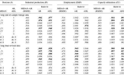
with an AR and an ADL, to determine whether monthly indi-cator information improves forecast accuracy. Table 1 gives the ratios of the RMSEs of the MIDAS–AR against the AR and ADL models. The table shows sizeable reductions in RMSE using MIDAS when monthly data are available on the current quarter; these are of the order of 20% when industrial produc-tion is the indicator for “nowcasts” andh=1/3 horizons (com-pared with the quarterly-frequency ADL). The RMSEs are cal-culated for output growth rates calcal-culated as 100 times the quar-terly difference of the natural log of GDP. So taking the MIDAS RMSE to be .4 for illustrative purposes, a RMSE ratio of the MIDAS to the ADL of .8 translates into respective RMSEs at annual rates of 1.6% and 2.0%, set against an average annual growth rate of 3.2% over the period.
Sizeable gains also are achieved when the indicator is capac-ity utilization for these horizons, whereas the differences be-tween MIDAS and the AR and ADL using employment are smaller. We also report average ratios across horizons, which confirm that MIDAS generally is no better (and often is worse) when no monthly information on the quarter is available.
In passing, we note that a comparison of the quarterly fre-quency ADL and AR models (with ADL/AR ratios obtained by dividing the MIDAS/AR ratio by the MIDAS/ADL ratio for each indicator in Table 1) presents a less upbeat picture of the usefulness of the indicators. Relative to an AR, the quarterly frequency ADL enhances accuracy only when employment is the indicator.
Table 1. Comparing the forecasting performance of MIDAS–AR with the AR and ADL using real-time end-of-sample vintage data and final-revised data
Horizon (h) Industrial production (IP) Employment (EMP) Capacity utilization (CU)
AR, ADL
MIDAS–AR (RMSE)
Ratio to
MIDAS–AR (RMSE)
Ratio to
MIDAS–AR (RMSE)
Ratio to
MIDAS AR ADL AR ADL AR ADL
Using end-of-sample vintage data
0 1 .444 .902 .877 .514 1.042 1.014 .452 .916 .895
1/3 1 .432 .876 .851 .487 .989 .962 .439 .890 .870
2/3 1 .516 1.046 1.017 .524 1.064 1.035 .515 1.045 1.021
1 1 .516 1.048 1.019 .493 1.001 .974 .492 .998 .975
4/3 2 .469 .937 .940 .512 1.024 1.018 .464 .928 .930
5/3 2 .512 1.024 1.027 .499 .998 .992 .513 1.025 1.028
2 2 .510 1.020 1.023 .496 .992 .987 .504 1.007 1.010
Av. 2 Av. 0 .451 .907 .896 .500 1.007 .991 .452 .909 .900
Av. 1 Av. 0 .514 1.035 1.022 .512 1.031 1.014 .514 1.035 1.024
Av. 0 Av. 0 .513 1.034 1.021 .495 .997 .980 .498 1.002 .992
Using final-revised data
0 1 .425 .869 .820 .471 .963 1.044 .440 .900 .840
1/3 1 .409 .837 .790 .472 .966 1.047 .438 .897 .837
2/3 1 .456 .932 .880 .474 .969 1.051 .484 .991 .925
1 1 .536 1.098 1.036 .477 .975 1.057 .521 1.067 .996
4/3 2 .459 .965 .964 .466 .981 .995 .469 .987 .984
5/3 2 .491 1.033 1.032 .472 .994 1.009 .495 1.043 1.039
2 2 .487 1.026 1.025 .479 1.008 1.023 .490 1.031 1.027
Av. 2 Av. 0 .435 .902 .874 .469 .973 1.021 .454 .942 .907
Av. 1 Av. 0 .473 .983 .952 .473 .981 1.029 .490 1.017 .979
Av. 0 Av. 0 .512 1.063 1.031 .478 .991 1.040 .506 1.049 1.010
NOTE: The entries (except the first column of each panel) are ratios of RMSE of MIDAS–AR to the AR and ADL. The RMSEs are computed using final-revised actual values of output growth for forecasts of 1985:Q2–2005:Q1. The ratios in bold imply that the null of equal RMSE is rejected at the 5% significance level using bootstrapped critical values. Av. 0 is the average RMSE when no information on the indicator in the current quarter is used for forecasting (h=1,2). Av. 1 is the equivalent when only 1 month on the current quarter is available (h=2/3, 5/3). Av. 2 is the same measure when 2 months of information are available (h=1/3, 4/3).
Clements and Galvão: Macroeconomic Forecasting With Mixed-Frequency Data 551
The exercise using final-revised vintage data allows us to cal-culate critical values to determine whether the gains that we observe from MIDAS at the shorter horizons are statistically significant. Following in the tradition of testing for equal pre-dictive ability of West (1996) and West and McCracken (1998) (also see the review in West 2006), we employ the test of equal forecast accuracy for multistep forecasts from nested models of Clark and McCracken (2005). The aim is to compare the fore-cast performance in population. Note that the MIDAS–AR nests both the AR and ADL models; it specializes to the ADL when
θ1=θ2=0 in (2). The null is that the quarterly frequency AR
(ADL) model forecasts are as accurate on RMSE as those of the MIDAS–AR (the unrestricted model), and the one-sided alter-native is that the AR (ADL) model forecasts are less accurate. Because the test has a limiting distribution that depends on the data, we adopt a bootstrap implementation of the test (similar to that of Kilian 1999). The boldface entries in the table indicate that the null of equal RMSE is rejected at the 5% level using the bootstrapped critical values, so that the gains from using MIDAS at the shorter horizons clearly are significant for both industrial production and capacity utilization.
Testing for equal predictive ability is more complicated in real-time forecasting exercises when there are data revisions across the vintages. Clark and McCracken (2007) showed that data revisions may affect the asymptotic behavior of tests of equal forecast accuracy and suggested a way to proceed using linear models estimated by least squares. It is unclear how use-ful these results are in our context. The natural solution of us-ing a bootstrap would require specification of the (unknown) revision process. For the forecasting comparisons based on the real-time use of end-of-sample and real-time vintage data, we simply report the relative sizes of the Root Mean Squared Fore-cast Errors (RMSFEs) and dispense with the use of formal tests of equal predictive ability.
Now consider the real-time end-of-sample vintage data. The results clearly indicate that IP and CU help predict output growth in real time when we have access to monthly data on the quarter being forecast. When only information on the pre-vious quarter is used, the indicators are of no value in real time. These results essentially match those obtained using final-revised data. In real time, the gains to MIDAS relative to the AR
disappear when EMP is the indicator, suggesting that the ap-parent gains from using EMP to predict output growth are not attainable in practice. In real time, the gains from using EMP at the quarterly frequency also disappear (i.e., comparison of the ADL against the AR). The boldface entries in the table indicate that the null of equal RMSE is rejected at the 5% level using the bootstrapped critical values calculated for the exercise using the final-revised data, but, as noted, the use of these critical values is questionable when there are data revisions. Nevertheless, it is apparent that MIDAS results in marked reductions in empirical RMSFEs in real time for the shorter horizons.
3.3 MIDAS–AR versus Other Methods of Exploiting Monthly Indicators
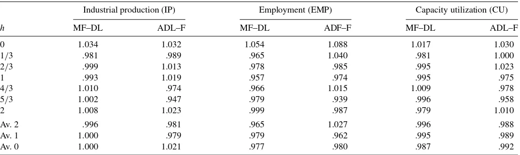
We compare the MIDAS–AR with other ways of using monthly indicator data, the MF–DL and the ADL–F described in Section 2.3, using end-of-sample vintage data. When all of the months of the quarter being forecast are known, ADL–F corresponds to a standard ADL, because data on the current quarter value of the indicator are available. Broadly speaking, the results given in Table 2 indicate that there is little to choose from between the models. The MF–DL and ADL–F are bet-ter than MIDAS for nowcasting (h=0), but when only 1 or 2 months of indicator data are available, MIDAS is generally at least as good (see the averages of the ratios across different hori-zons). Overall, except whenh=0, the performance of MIDAS is promising compared with that of other simple methods of us-ing monthly indicators to forecast quarterly growth. However, Koenig et al. (2003) showed that using real-time vintage data improves the forecast accuracy of MF–DL and advocated this approach to forecast accuracy comparisons. The next section reports a comparison using real-time vintage data.
3.4 MIDAS–AR and Other Methods of Exploiting Monthly Indicators With Real-Time Vintage Data
Conducting the forecasting exercise using real-time vintage data supports the finding that monthly indicator information helps predict output growth, especially at shorter horizons. This
Table 2. Comparing the forecasting performance of MIDAS–AR with ADL–F and MF–DL using real-time end-of-sample vintage data
Industrial production (IP) Employment (EMP) Capacity utilization (CU)
h MF–DL ADL–F MF–DL ADF–F MF–DL ADL–F
0 1.034 1.032 1.054 1.088 1.017 1.030
1/3 .981 .989 .965 1.040 .981 1.000
2/3 .999 1.013 .978 .985 .995 1.023
1 .993 1.019 .957 .974 .995 .975
4/3 1.010 .974 .966 1.015 1.009 .978
5/3 1.002 .947 .979 .939 .996 .958
2 1.008 1.023 .999 .987 .979 1.010
Av. 2 .996 .981 .965 1.027 .996 .988
Av. 1 1.000 .979 .979 .962 .995 .989
Av. 0 1.000 1.021 .977 .980 .987 .992
NOTE: The entries are ratios of the MIDAS–AR RMSEs to the RMSEs of the stated models. Av. 0 is the average RMSE when no information on the indicator in the current quarter is used for forecasting (h=1,2). Av. 1 is the equivalent when only 1 month on the current quarter is available (h=2/3, 5/3). Av. 2 is the same measure when 2 months of information are available (h=1/3, 4/3).
Table 3. Comparing the forecasting performance of MIDAS–AR with that of MF–DL, ADL–F, and AR using real-time vintage data and end-of-sample vintage data
Industrial production (IP) Employment (EMP) Capacity utilization (CU)
h MIDAS–AR MF–DL ADL–F MIDAS–AR MF–DL ADL–F MIDAS–AR MF–DL ADL–F AR
Real-time vintage data/end-of-sample vintage data
0 .971 1.005 .990 .961 1.034 .952 .996 1.041 .960
1/3 .974 .971 .962 .973 .988 .970 1.011 1.034 .971
2/3 .993 .988 1.124 .959 .968 .937 1.027 1.029 1.066
1 1.018 1.048 .984 1.036 1.029 1.008 1.098 1.105 .991 1.035
4/3 1.028 1.066 1.000 1.001 1.001 .995 1.019 1.023 .963
5/3 .996 1.024 1.071 1.015 1.018 .965 1.014 1.042 1.069
2 1.029 1.050 1.014 1.029 1.065 1.029 1.020 1.021 .991 1.012
Ratio of MIDAS–AR with real-time vintage data to
AR MF–DL ADL–F AR MF–DL ADL–F AR MF–DL ADL–F
Av. 2 .890 .978 1.001 .972 .958 1.031 .902 .983 .995
Av. 1 1.006 .989 .888 .993 .973 .998 1.033 .981 .961
Av. 0 1.034 .976 1.046 1.006 .965 .994 1.038 .984 1.029
NOTE: The entries in the top part are RMSE ratios of the stated model estimated with real-time vintage data to the same model but estimated with end-of-sample vintage data. The entries in the bottom part are ratios of the MIDAS–AR RMSEs to the RMSEs of the stated models using real-time vintage data. Av. 0 is the average RMSE when no information on the indicator in the current quarter is used for forecasting (h=1,2). Av. 1 is the equivalent when only 1 month on the current quarter is available (h=2/3, 5/3). Av. 2 is the same measure when 2 months of information are available (h=1/3, 4/3).
is partly because the forecast performance of the AR wors-ens relative to when end-of-sample data are used (by just over 3% on RMSE ath=1), whereas the performance of MIDAS and ADL–F generally improves. Table 3 gives the ratios of the RMSEs when using real-time vintage data to using end-of-sample vintage data for each monthly model and the AR. The net result of these changes is that MIDAS is more accurate than the AR for h=0, 1/3 for all three indicators. The table also shows that for horizons with 2 months of indicator information available (the “Av. 2” row), the gains to MIDAS are of the order of a 10% reduction in RMSE for IP and CU and a 3% reduction for EMP.
It is worth remarking that MIDAS is generally as good at the shorter horizons as the popular two-step approach to the incor-poration of monthly information exemplified by the ADL–F, except when the indicator is EMP, and is almost always supe-rior to the MF–DL.
3.5 Forecast Combination
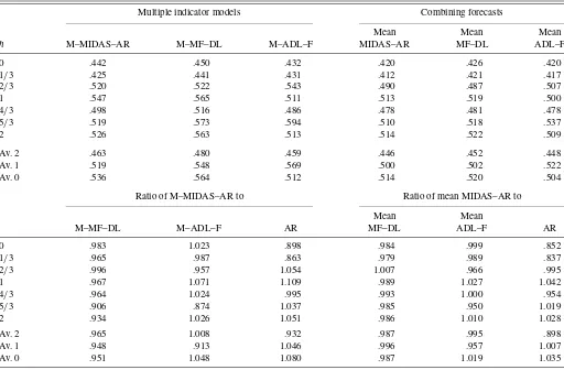
Table 4 compares models that include all three indicators (which have the prefix “M–,” for multiple) with equal-weighted combinations of the individual indicator models. The results in-dicate that the MIDAS model is clearly preferred to MF–DL. It also beats ADL–F when the horizon is not an integer multiple of quarters, that is, for those horizons when ADL–F relies on monthly forecasts to construct quarterly observations. Combin-ing forecasts is better than combinCombin-ing indicators within a sin-gle model (as is often the case; see, e.g., Clements and Galvão 2006), but the combinations of the MIDAS models’ forecasts are generally at least as good as the combinations of the fore-casts from the other two models.
4. CONCLUSIONS
In recent years, increasing use has been made of monthly indicator information to generate forecasts of quarterly macro
aggregates, such as GDP growth. We have investigated whether the MIDAS approach of Ghysels et al. (2004, 2006b) can be successfully adapted to short-term forecasts of output growth, given that it has hitherto been used for forecasting financial variables with daily observations. A typical feature of quarterly macroeconomic time series is that they often can be reasonably well modeled by AR processes. To capture this characteristic of macro data, we extended the distributed-lag MIDAS specifica-tion to include an AR term (the MIDAS–AR) and showed how this model can be applied in a forecasting context.
Recent research suggests that the predictive content of in-dicator information must be assessed in an exercise that mir-rors a “real-time-forecasting environment,” and that using final-revised data may misleadingly suggest that the indicators are better than what could be achieved with the data available at the time. We conducted a traditional real-time forecasting ex-ercise that exploits the monthly vintages of the indicators and the quarterly vintages of output growth and that is consistent with the timing of the releases of the different data vintages. This permits a comprehensive and valid appraisal of the use-fulness of monthly information in real time. We found that the use of monthly indicator information resulted in sizeable reduc-tions in RMSE for short-horizon forecasts when within-quarter monthly data on industrial production and capacity utilization are used.
We also evaluated the suggestion by Koenig et al. (2003) to base the real-time forecasting exercise on real-time vintage data as opposed to end-of-sample vintage data. We did so for a range of forecast horizons, from the “nowcasts” considered by Koenig et al. up to the 2-quarter horizon, in steps of 1 month. The use of real-time vintage data serves to strengthen our finding that within-quarter monthly indicator information can result in marked improvements in forecast performance. MIDAS fares well relative to the other models that use monthly information. Coupled with its flexibility and ease of use relative to methods
Clements and Galvão: Macroeconomic Forecasting With Mixed-Frequency Data 553
Table 4. Comparing combinations of indicators: M–MIDAS–AR, M–ADL–F, M–MF–DL, and means of forecasts using real-time vintage data
Multiple indicator models Combining forecasts
Mean Mean Mean
h M–MIDAS–AR M–MF–DL M–ADL–F MIDAS–AR MF–DL ADL–F
0 .442 .450 .432 .420 .426 .420
1/3 .425 .441 .431 .412 .421 .417
2/3 .520 .522 .543 .490 .487 .507
1 .547 .565 .511 .513 .519 .500
4/3 .498 .516 .486 .478 .481 .478
5/3 .519 .573 .594 .510 .518 .537
2 .526 .563 .513 .514 .522 .509
Av. 2 .463 .480 .459 .446 .452 .448
Av. 1 .519 .548 .569 .500 .502 .522
Av. 0 .536 .564 .512 .514 .520 .504
Ratio of M–MIDAS–AR to Ratio of mean MIDAS–AR to
Mean Mean
M–MF–DL M–ADL–F AR MF–DL ADL–F AR
0 .983 1.023 .898 .984 .999 .852
1/3 .965 .987 .863 .979 .989 .837
2/3 .996 .957 1.054 1.007 .966 .995
1 .967 1.071 1.109 .989 1.027 1.042
4/3 .964 1.024 .995 .993 1.000 .954
5/3 .906 .874 1.037 .985 .950 1.019
2 .934 1.026 1.051 .986 1.010 1.028
Av. 2 .965 1.008 .932 .987 .995 .898
Av. 1 .948 .913 1.046 .996 .957 1.007
Av. 0 .951 1.048 1.080 .987 1.019 1.035
NOTE: The entries in the top part are RMSEs. The bottom part records the RMSE ratios of MIDAS to the stated model. Av. 0 is the average RMSE when no information on the indicator in the current quarter is used for forecasting (h=1,2). Av. 1 is the equivalent when only 1 month of information for the current quarter is available (h=2/3, 5/3). Av. 2 is the same measure when 2 months of information are available (h=1/3, 4/3).
that involve generation of forecasts of explanatory variables of-fline, the MIDAS–AR would appear to be a useful addition to the sets of models and methods that exploit monthly indicators for the short-term forecasting of macroaggregates.
ACKNOWLEDGMENTS
The authors are grateful to the editor, an associate editor, and three anonymous referees for helpful comments and guidance. They also acknowledge helpful comments from participants at the International Symposium of Forecasting in Santander, June 2006.
[Received September 2005. Revised November 2007.]
REFERENCES
Boivin, J., and Ng, S. (2005), “Understanding and Comparing Factor-Based Forecasts,”International Journal of Central Banking, 1, 117–151. Clark, T. E., and McCracken, M. W. (2005), “Evaluating Direct Multi-Step
Forecasts,”Econometric Reviews, 24, 369–404.
(2007), “Tests of Equal Predictive Ability With Real-Time Data,” dis-cussion paper, Federal Reserve Bank of Kansas City, Economic Research Dept.
Clements, M. P., and Galvão, A. B. (2006), “Combining Predictors and Com-bining Information in Modelling: Forecasting U.S. Recession Probabilities and Output Growth,” inNonlinear Time Series Analysis of Business Cycles: Contributions to Economic Analysis Series, eds. C. Milas, P. Rothman, and D. van Dijk, Amsterdam: Elsevier, pp. 55–73.
Clements, M. P., and Harvey, D. I. (2008), “Forecasting Combination and Encompassing,” inPalgrave Handbook of Econometrics, Vol. 2: Applied Econometrics, eds. T. C. Mills and K. Patterson, Hampshire: Palgrave Macmillan, forthcoming.
Croushore, D., and Stark, T. (2001), “A Real-Time Data Set for Macroecono-mists,”Journal of Econometrics, 105, 111–130.
Dhrymes, P. J. (1971),Distributed Lags: Problems of Estimation and Formula-tion, San Francisco: Holden-Day.
Diebold, F. X., and Lopez, J. A. (1996), “Forecast Evaluation and Combina-tion,” inHandbook of Statistics, Vol. 14, eds. G. S. Maddala and C. R. Rao, Amsterdam: North-Holland, pp. 241–268.
Diebold, F. X., and Rudebusch, G. D. (1991), “Forecasting Output With the Composite Leading Index: A Real-Time Analysis,”Journal of the American Statistical Association, 86, 603–610.
Faust, J., Rogers, J. H., and Wright, J. H. (2003), “Exchange Rate Forecasting: The Errors We’ve Really Made,”Journal of International Economic Review, 60, 35–39.
Ghysels, E., and Wright, J. (2006), “Forecasting Professional Forecasters,” Fi-nance and Economics Discussion Series 2006-10, Board of Governors of the Federal Reserve System (U.S.), Washington, DC.
Ghysels, E., Santa-Clara, P., and Valkanov, R. (2004), “The MIDAS Touch: Mixed Data Sampling Regression Models,” CIRANO Working Papers 2004s-20, CIRANO, Montreal, Canada.
(2006a), “Predicting Volatility: Getting the Most Out of Return Data Sampled at Different Frequencies,”Journal of Econometrics, 131, 59–95. Ghysels, E., Sinko, A., and Valkanov, R. (2006b), “MIDAS Regressions:
Fur-ther Results and New Directions,”Econometric Reviews, 26, 53–90. Hendry, D. F., and Mizon, G. E. (1978), “Serial Correlation as a Convenient
Simplification, Not a Nuisance: A Comment on a Study of the Demand for Money by the Bank of England,”Economic Journal, 88, 549–563. Reprinted in Hendry, D. F. (1993, 2000),Econometrics: Alchemy or Science?Oxford, U.K.: Blackwell, and Oxford University Press.
Joutz, F., and Stekler, H. O. (2000), “An Evaluation of the Predictions of the Federal Reserve,”International Journal of Forecasting, 16, 17–38.
Karamouzis, N., and Lombra, N. (1989), “Federal Reserve Policymaking: An Overview and Analysis of the Policy Process,”Carnegie Rochester Confer-ence Series on Public Policy, 30, 7–62.
Kilian, L. (1999), “Exchange Rates and Monetary Fundamentals: What Do We Learn From Long-Horizon Regressions,”Journal of Applied Econometrics, 14, 491–510.
Koenig, E. F., Dolmas, S., and Piger, J. (2003), “The Use and Abuse of Real-Time Data in Economic Forecasting,”Review of Economics and Statistics, 85, 618–628.
Miller, P. J., and Chin, D. M. (1996), “Using Monthly Data to Improve Quar-terly Model Forecasts,”Federal Reserve Bank of Minneapolis Quarterly Re-view, 20, 16–33.
Newbold, P., and Harvey, D. I. (2002), “Forecasting Combination and Encom-passing,” inA Companion to Economic Forecasting, eds. M. P. Clements and D. F. Hendry, Oxford, U.K.: Blackwell, pp. 268–283.
Orphanides, A. (2001), “Monetary Policy Rules Based on Real-Time Data,”
American Economic Review, 91, 964–985.
Orphanides, A., and van Norden, S. (2005), “The Reliability of Inflation Fore-casts Based on Output Gaps in Real Time,”Journal of Money, Credit and Banking, 37, 583–601.
Rünstler, G., and Sédillot, F. (2003), “Short-Term Estimates of Euro Area Real GDP by Means of Monthly Data,” Working Paper 276, European Central Bank.
Schumacher, C., and Breitung, J. (2006), “Real-Time Forecasting of GDP Based on a Large Factor Model With Monthly and Quarterly Data,” Dis-cussion Paper 33/2006, Deutsche Bundesbank.
Sims, C. A. (1974), “Distributed Lags,” inFrontiers of Quantitative Economics, Vol. 2, eds. M. D. Intriligator and D. A. Kendrick, Amsterdam: North-Holland, Chap. 5.
Stock, J. H., and Watson, M. W. (2003), “How Did Leading Indicator Forecasts Perform During the 2001 Recession,”Federal Reserve Bank of Richmond Economic Quarterly, 89/3, 71–90.
Timmermann, A. (2006), “Forecast Combinations,” inHandbook of Economic Forecasting, Vol. 1, eds. G. Elliott, C. Granger, and A. Timmermann, Ams-terdam: Elsevier, pp. 135–196.
West, K. D. (1996), “Asymptotic Inference About Predictive Ability,” Econo-metrica, 64, 1067–1084.
(2006), “Forecasting Evaluation,” inHandbook of Economic Forecast-ing, Vol. 1, eds. G. Elliott, C. Granger, and A. Timmermann, Amsterdam: Elsevier, pp. 99–134.
West, K. D., and McCracken, M. W. (1998), “Regression-Based Tests of Pre-dictive Ability,”International Economic Review, 39, 817–840.
Zheng, I. Y., and Rossiter, J. N. (2006), “Using Monthly Indicators to Predict Quarterly GDP,” Working Paper 2006-26, Bank of Canada.