07350015%2E2013%2E792264

(1)

Full Terms & Conditions of access and use can be found at

http://www.tandfonline.com/action/journalInformation?journalCode=ubes20

Download by: [Universitas Maritim Raja Ali Haji] Date: 11 January 2016, At: 22:11

Journal of Business & Economic Statistics

ISSN: 0735-0015 (Print) 1537-2707 (Online) Journal homepage: http://www.tandfonline.com/loi/ubes20

Comment

Brendan Kline & Elie Tamer

To cite this article: Brendan Kline & Elie Tamer (2013) Comment, Journal of Business & Economic Statistics, 31:3, 276-279, DOI: 10.1080/07350015.2013.792264

To link to this article: http://dx.doi.org/10.1080/07350015.2013.792264

Published online: 22 Jul 2013.

Submit your article to this journal

Article views: 256

(2)

276 Journal of Business & Economic Statistics, July 2013

Comment

Brendan K

LINE

Department of Economics, University of Texas at Austin, Austin, TX 78712 (brendan.kline@austin.utexas.edu)

Elie T

AMER

Department of Economics, Northwestern University, Evanston, IL 60208 (tamer@northwestern.edu)

1. INTRODUCTION

The article by Goldsmith-Pinkham and Imbens (2013) is an

interesting contribution to the literature on social interactions. An important contribution of their article is to provide some answers to the question: what features of models of social in-teractions are empirically relevant? This question concerns the relationship between the true data-generating process and the model used by the econometrician. In our comment on their ar-ticle, we ask an alternative question: how should policy makers use the estimates from the linear-in-means model? This question concerns the relationship between the model used by the econo-metrician and policy interventions. The scope of our comment extends beyond the article by Goldsmith-Pinkham and Imbens (2013) to address this issue in the general linear-in-means model literature.

We first derive standard marginal effects of a change in a covariate. These are complicated functions of the model param-eters. This suggests that it may be useful for applications of the linear-in-means model to report these policy relevant param-eters. Another interpretation views the linear-in-means model as a best response function from some game. This gives an autonomous interpretation to the parameters and uncovers the mechanisms underlying the interaction. This approach, though natural in economics, is based on a very particular model of interaction.

2. POLICY-RELEVANT PARAMETERS IN THE

LINEAR-IN-MEANS MODEL

The specification of the linear-in-means model used by Goldsmith-Pinkham and Imbens (2013) is that, for a group ofN

individuals,

Y=ιNβ0+Xβx+GYβy+GXβx+η,

where Y _{is the} N×1 vector of outcomes, ιN is the N×1

vector of ones,X_{is the}N×Kmatrix of observable covariates,

G_{is the}N×N row-normalized adjacency matrix, andηis the

N×1 vector of unobservables. The parametersβ0,βx,βy, and

βxare the unknown parameters of the model, which are 1×1,

K×1, 1×1, andK×1, respectively. The setup of this model is discussed in more detail in Goldsmith-Pinkham and Imbens (2013), as well as many related articles, and so we do not provide further explanation here.

The following theorem, and subsequent discussion, concerns

the marginal effects of X_on Y _{that accounts for the}

reequi-libration of the outcomes Y_{after a policy intervention affects}

X_{. The reequilibration is a consequence of the fact that}Y_are

simultaneously determined.

The theorem and discussion presumes that the parameters are known, but of course the identification of these parameters is a subtle question that has been addressed, for example, by

Manski (1993), Graham and Hahn (2005), Lee (2007),

Gra-ham (2008), Bramoull´e, Djebbari, and Fortin (2009), and De Giorgi, Pellizzari, and Redaelli (2010). The current article by

Goldsmith-Pinkham and Imbens (2012) provides some

empiri-cal results related to different extensions of the linear-in-means model. In the following theorem, letei be the 1×N unit row

vector with a 1 in theith column.

Theorem 2.1. Suppose that the model is

Y=ιNβ0+Xβx+GYβy+GXβx+η,

withE(η|X,G₎=0. Suppose thatϒ≡I_N_×_N₋Gβyis

nonsin-gular (see Remark 2.1).

Then, the marginal effects ofX_onE(yi|X,G) are given by

βxeiϒ−1+βxeiϒ−1G,

where the marginal effect of thekth covariate of individualjis the (k, j) entry of this matrix.

In the special case thatG_{represents the complete network}

(i.e., each off-diagonal entry ofG_is 1

N−1) as in the “standard”

linear-in-means model, the effects of the various elements ofX

onE(yi|X,G) are the following:

Now, in the special case that G _{represents the}

com-plete network, writeϒ=u1IN×N+u21N×N, whereu1=1+

July 2013, Vol. 31, No. 3 DOI:10.1080/07350015.2013.792264

(3)

1_N_×_N₎₌βx(_u1₁ei−_u₁₍_u₁u₊2_{N u}₂₎11×N). Also, it holds that ϒ−1

This is the K×N matrix of marginal effects. In

particu-lar, (βx_u1

1 +βx

g1

u1)ei is the K×N matrix, which is 0 in any

element that is not in the ith column, and the ith column is

βx_u1

Remark 2.1 (Nonsingularity ofϒ). A sufficient condition for the nonsingularity ofϒ is|βy|<1. Note thatϒ is the matrix

with 1’s along the diagonal, and that the row sum of the absolute values of the off-diagonal entries is|βy|. If|βy|<1,ϒis strictly

diagonally dominant, so is nonsingular.

This result can be understood by recognizing that the effect of

X_onY_{can be decomposed into three effects. The “exogenous}

nonsocial interaction” effect is the fact that manipulating the observable covariates of individualiaffects the outcome of in-dividuali, according to the parameterβx. The “exogenous social

interaction” effect is the fact that manipulating the observable covariates of individualj =iaffects the outcomes of the peers of individualj, according to the parameterβx. Finally, the

“en-dogenous social interaction” effect is the fact that the outcomes

Y_{are simultaneously determined, according to the parameter}

βy. If a policy experiment is allowed to cause a reequilibration

in the outcomes, then all three of these effects appear in the marginal effect ofX_onY_.

Roughly, the parameters βx and βx can be directly

inter-preted as the effects of the observable covariates holding fixed the outcomes of an individual’s peers. Such “partial equilib-rium” effects are certainly of interest theoretically, particularly to understand the mechanism by which the social interaction works. However, it is important to note that such an interpre-tation does require some nontrivial theoretical underpinnings. In particular, it requires that the econometrician be willing

to give an autonomous interpretation to each equation in the

modelY=ιNβ0+Xβx+GYβy+GXβx+η,which are the

equationsyi=β0+xiβx+[GY]iβy+[GX]iβx+ηi. An

au-tonomous interpretation of these equations requires that each equation be valid as a stand-alone equation, even for values

of Y_{that are not in equilibrium according to the full model.}

See also, for example, Goldberger (1991) or Wooldridge (2001)

for a discussion of autonomous interpretation of equations in simultaneous equations models.

For example, yi =β0+xiβx+[GY]iβy+[GX]iβx+ηi

could be given an autonomous interpretation if the

econome-trician views the model as determining Y _{as the fixed point}

of the best response functions from some game. In that case,

β0+xiβx+[GY]iβy+[GX]iβx+ηi is the best response of

individual i to the “decisions” of the other individuals in the group; this best response depends also on the other variables in the model. The important fact is that this autonomous interpre-tation (i.e., the interpreinterpre-tation of equation ias a best response function) requires that the same interpretation obtains even in a partial equilibrium, where the value ofY_{“plugged into” the}

equation is not an equilibrium outcome. Then, βx andβx

de-scribe how these best responses depend on the observable covari-ates. Although a formal result along these lines is not presented here because of space constraints, it is generally known that a game with quadratic utility functions has linear best response functions. In related work, Kline and Tamer (2012) showed how to nonparametrically partially identify the best response func-tions in games. See also, for example, Kline (2012) for more on identification of models of games that could be used to specifi-cally model a social interaction, in particular allowing a network of peer relationships. More generally, see, for example, Tamer (2003).

3. NUMERICAL EXAMPLE

It remains, of course, an empirical question whether these policy relevant parameters differ significantly from the param-eters of the linear-in-means model directly. In particular, when

βy=0, and whenGrepresents the complete network, it follows

thatλ=1,ψ=0, andω= _N1₋₁, so that the policy relevant pa-rameters are simply the papa-rameters of the model directly. Of course, settings whereβy=0 are settings where the social

in-teraction in outcomes is not present, and are therefore not of particular interest. Consequently, we provide a brief set of nu-merical examples suggesting that the policy relevant parameters for various specifications of the parameters of the linear-in-means model can differ substantially from the parameters of the linear-in-means model directly.

In these numerical examples we set K=1, so that there

is only one observable covariate. Also, we set N=20, and

suppose thatG_{represents the complete network, so we have in}

mind the application of the “standard” linear-in-means model to a classroom setting.

The policy relevant parameters we consider are∂E(yi|X,G)

∂xik and

(N−1)∂E(yi|X,G)

∂xj k . The former is the marginal effect on an

indi-vidual’s outcome of that indiindi-vidual’s own observable covariatek. The latter is the marginal effect on an individual’s outcome of an equal increase in all of the observable covariateskof that individ-ual’s peers. This may be roughly interpreted to be the marginal effect of “increasing the average” of the peers’ observable co-variatesk; however, evidently in general this interpretation re-quires some caution because the distribution of the increase among the peers can matter depending on the network structure. More formally, writeX₌X˜ ₊CiT, whereCiis theN×1

col-umn vector that has 1’s in every element except for theith row,

(4)

278 Journal of Business & Economic Statistics, July 2013

Table 1. Policy relevant parameters, I

βy βx βx ∂E(yi| X,G)

∂xik (N−1)

∂E(yi|X,G)

∂xj k

0.10 0.60 0.05 0.6006 0.1216

0.10 0.60 0.10 0.6009 0.1768

0.10 0.60 0.15 0.6012 0.2321

0.10 0.70 0.05 0.7007 0.1326

0.10 0.70 0.10 0.7010 0.1879

0.10 0.70 0.15 0.7013 0.2432

0.10 0.80 0.05 0.8008 0.1437

0.10 0.80 0.10 0.8010 0.1990

0.10 0.80 0.15 0.8013 0.2542

0.15 0.60 0.05 0.6013 0.1634

0.15 0.60 0.10 0.6018 0.2218

0.15 0.60 0.15 0.6022 0.2801

0.15 0.70 0.05 0.7014 0.1809

0.15 0.70 0.10 0.7019 0.2393

0.15 0.70 0.15 0.7023 0.2977

0.15 0.80 0.05 0.8016 0.1984

0.15 0.80 0.10 0.8020 0.2568

0.15 0.80 0.15 0.8025 0.3152

0.20 0.60 0.05 0.6022 0.2103

0.20 0.60 0.10 0.6029 0.2721

0.20 0.60 0.15 0.6035 0.3340

0.20 0.70 0.05 0.7025 0.2350

0.20 0.70 0.10 0.7031 0.2969

0.20 0.70 0.15 0.7038 0.3587

0.20 0.80 0.05 0.8027 0.2598

0.20 0.80 0.10 0.8034 0.3216

0.20 0.80 0.15 0.8040 0.3835

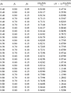
Table 2. Policy relevant parameters, II

βy βx βx ∂E(yi| X,G)

∂xik (N−1)

∂E(yi|X,G)

∂xj k

0.40 0.60 0.05 0.6100 0.4734

0.40 0.60 0.10 0.6117 0.5550

0.40 0.60 0.15 0.6134 0.6366

0.40 0.70 0.05 0.7113 0.5387

0.40 0.70 0.10 0.7131 0.6203

0.40 0.70 0.15 0.7148 0.7019

0.40 0.80 0.05 0.8127 0.6040

0.40 0.80 0.10 0.8144 0.6856

0.40 0.80 0.15 0.8162 0.7672

0.50 0.60 0.05 0.6179 0.6821

0.50 0.60 0.10 0.6205 0.7795

0.50 0.60 0.15 0.6231 0.8769

0.50 0.70 0.05 0.7205 0.7795

0.50 0.70 0.10 0.7231 0.8769

0.50 0.70 0.15 0.7256 0.9744

0.50 0.80 0.05 0.8231 0.8769

0.50 0.80 0.10 0.8256 0.9744

0.50 0.80 0.15 0.8282 1.0718

0.60 0.60 0.05 0.6314 0.9936

0.60 0.60 0.10 0.6352 1.1148

0.60 0.60 0.15 0.6390 1.2360

0.60 0.70 0.05 0.7360 1.1390

0.60 0.70 0.10 0.7398 1.2602

0.60 0.70 0.15 0.7436 1.3814

0.60 0.80 0.05 0.8406 1.2844

0.60 0.80 0.10 0.8444 1.4056

0.60 0.80 0.15 0.8482 1.5268

where the entry is 0. The 1×Krow vectorThas generic

ele-menttk. Then, as in the proof of the main theorem, ∂E(yi|

X,G)

∂T =

(βxeiϒ−1+βxeiϒ−1G)Ci. Consequently, the marginal effect

oftk, which can be interpreted to be the marginal effect of

in-creasing the observable covariatekof all of an individual’s peers by the same amount, is simply the sum of the marginal effects of each specific peer’s observable covariatek. In the case whereG

represents the complete network, this is simply (N−1) times the marginal effect of any given peer’s observable covariates, since all such effects are equal. So, for the first marginal ef-fect, we report Equation (1) from Theorem 2.1; for the second marginal effect, we report (N−1) times Equation (2).

Table 1takes the general magnitudes of the parameters from Goldsmith-Pinkham and Imbens (2013). The table suggests that the marginal effect of an individual’s own observable covariate

is well approximated byβx. However, the marginal effect of

an individual’s peers’ observable covariates is not well approx-imated by βx. Table 2 shows the results for larger, but still

plausible, values ofβy. There, neither marginal effect is well

approximated by the “corresponding”β parameter, and in

par-ticular the marginal effect of an individual’s peers’ observable covariates is much larger thanβx.

4. CONCLUSIONS

If marginal effects are the objects of interest, then applica-tions of the linear-in-means model should consider reporting these policy relevant functions of the parameters in addition to the parameters of the model directly. Similarly, applications of extensions of the linear-in-means model should consider report-ing the policy relevant functions of the parameters appropriate for that extension. An alternative is to give an autonomous in-terpretation to the equations of the linear-in-means model. One natural autonomous interpretation is to interpret the equations as best response functions.

The existence of these two possibilities, either to use the re-sults of Theorem 2.1 or to give an autonomous interpretation to the equations of the linear-in-means model, raises a tradeoff. The first possibility is “automatic” given the structure of the linear-in-means model, but may not answer questions about “partial equilibrium.” The second possibility requires the econometri-cian to make additional assumptions that justify the autonomous interpretation of each equation, but does answer questions about “partial equilibrium.”

ACKNOWLEDGMENTS

Authors greatly appreciate the support from the National Sci-ence Foundation. The authors are responsible for any errors.

REFERENCES

Bramoull´e, Y., Djebbari, H., and Fortin, B. (2009), “Identification of Peer Effects

Through Social Networks,”Journal of Econometrics, 150, 41–55. [276]

De Giorgi, G., Pellizzari, M., and Redaelli, S. (2010), “Identification of

So-cial Interactions Through Partially Overlapping Peer Groups,”American

Economic Journal: Applied Economics, 2, 241–275. [276]

(5)

Goldberger, A. (1991),A Course in Econometrics, Cambridge, MA: Harvard University Press. [277]

Goldsmith-Pinkham, P., and Imbens, G. W. (2013), “Social Networks and the Identification of Peer Effects,”Journal of Business and Economic Statistics, 31, 253–264. [276,278]

Graham, B. (2008), “Identifying Social Interactions Through Conditional

Vari-ance Restrictions,”Econometrica, 76, 643–660. [276]

Graham, B., and Hahn, J. (2005), “Identification and Estimation of the

Linear-in-Means Model of Social Interactions,”Economics Letters, 88,

1–6. [276]

Kline, B. (2012), “Identification of Complete Information Games,” Working Paper. [277]

Kline, B., and Tamer, E. (2012), “Bounds for Best Response Functions in Binary

Games,”Journal of Econometrics, 166, 92–105. [277]

Lee, L. (2007), “Identification and Estimation of Econometric Models With

Group Interactions, Contextual Factors and Fixed Effects,” Journal of

Econometrics, 140, 333–374. [276]

Manski, C. (1993), “Identification of Endogenous Social Effects: The Reflection

Problem,”Review of Economic Studies, 60, 531–542. [276]

Tamer, E. (2003), “Incomplete Simultaneous Discrete Response Model

With Multiple Equilibria,” Review of Economic Studies, 70, 147–

165. [277]

Wooldridge, J. (2001),Econometric Analysis of Cross Section and Panel Data,

Cambridge, MA: The MIT Press. [277]

Rejoinder

Paul G

OLDSMITH

-P

INKHAM

Department of Economics, Harvard University, Cambridge, MA 02138 (pgoldsm@fas.harvard.edu)

Guido I

MBENS

Graduate School of Business, Stanford University, Stanford, CA 94305, and NBER (imbens@stanford.edu)

First of all, we thank the Coeditors again for inviting us to present the article and for organizing such a distinguished group of researchers to comment on our work. We would also like to thank these individuals for their thoughtful discussion. These comments contain a great number of interesting questions and suggestions for future research, more than we can hope to address in our response. This partly reflects the fertility of this area of study, and we hope and suspect that the comments will stimulate further research.

A general issue raised in three of the comments concerns the focus on model parameters versus specific policy interventions. Jackson stresses the importance of being very explicit about the specific effects of interest, while Manski takes issue with our claim that “the main object of interest is the effect of peers’ outcomes on own outcomes” and points out that identification of the structural parameters is not the same as identification of the treatment responses. Relatedly, Kline and Tamer raise the issue of the interpretation of the parameters and their link to policy interventions.

Here, we were less careful than we should have been. Ul-timately, we agree wholeheartedly with these comments and withdraw the claim to which Manski objects. Manski’s linear-in-means example illustrates nicely the pitfalls of focusing solely on identifying parameters rather than policies, and we believe this is an important issue. Too often econometricians focus solely on the particular parameters in their models without re-lating them to interpretable and feasible interventions. With this objective in mind, Kline and Tamer focus on the effect of a change in either one’s own or others’ covariate values on the out-come of interest. They demonstrate how these measured effects are related in potentially complicated ways to the parameters of the model.

In the area of industrial organization, it is often the norm to report the effects of specific counterfactuals or policy inter-ventions, while in other areas of empirical economic research, it is much less common. In peer effects models, there are

di-rect policy interventions to consider, but there are also other policies whose effects are complicated functions of the model parameters. For example, in the context of a network formation model, Christakis et al. (2010) considered the effect of chang-ing features of the assignment to classes on the formation of friendships. Given our setup, one could envision a policy af-fecting friendship formation that was enacted with students’ grades in mind. In sum, we agree with the recommendation that researchers should routinely assess the effects of specific and relevant interventions rather than simply report parameter estimates.

Kline and Tamer also study the interpretation of the model parameters themselves and show how they can be interpreted as “best responses” in a game. This greatly improves the inter-pretability of these parameters, although ultimately we would still stress the importance of focusing on the effect of interven-tions rather than the parameters themselves. In some cases, it seems likely that the peer effects model is attempting to capture the effects of a “social multiplier” through a specification that reflects the researcher’s ignorance about the particular chan-nels by which this interaction occurs. However, we agree with both Jackson and Sacerdote’s view that a researcher should be modeling the specific type of social interaction she hopes to find. Interestingly, as Manski points out in his comment and

in Manski (2013), even researchers fortunate enough to have

randomized interventions will have to think hard about how to model the social interaction.

Bramoull´e raises important issues regarding the type of en-dogeneity we allow for in our model, discusses some identifica-tion quesidentifica-tions, and offers some suggesidentifica-tions on estimaidentifica-tion and on modeling heterogeneity in peer effects. It is interesting as a

July 2013, Vol. 31, No. 3 DOI:10.1080/07350015.2013.792260